
Concept explainers
Videos
The article “Photocharge Effects in Dye Sensitized Ag[Br, I] Emulsions at Millisecond
![Chapter 13, Problem 60CR, The article Photocharge Effects in Dye Sensitized Ag[Br, I] Emulsions at Millisecond Range Exposures](https://content.bartleby.com/tbms-images/9781337793612/Chapter-13/images/93612-13-60cr-question-digital_image_001.png)
- a. Construct a
scatterplot of the data. What does it suggest? - b. Assuming that the simple linear regression model is appropriate, obtain the equation of the estimated regression line.
- c. How much of the observed variation in peak photovoltage can be explained by the model relationship?
- d. Predict peak photovoltage when percent absorption is 19.1, and compute the value of the corresponding residual.
- e. The authors claimed that there is a useful linear relationship between the two variables. Do you agree? Carry out a formal test.
- f. Give an estimate of the average change in peak photovoltage associated with a 1 percentage point increase in light absorption. Your estimate should convey information about the precision of estimation.
- g. Give an estimate of mean peak photovoltage when percentage of light absorption is 20, and do so in a way that conveys information about precision.
a.
Construct a scatterplot for the data and explain what it suggests.
Explanation of Solution
Calculation:
The given data are on percentage of light absorption (x) and peak photo voltage (y).
If the scatterplot of the data shows a linear pattern, and the vertical variability of points does not appear to be changing over the range of x values in the sample, then it can be said that the data is consistent with the use of the simple linear regression model.
Software procedure:
Step-by-step procedure to obtain the scatterplot using MINITAB software:
- Choose Graph > Scatter plot.
- Select Simple.
- Click OK.
- Under Y variables, enter the column of y.
- Under X variables, enter the column of x.
- Click OK.
The output using MINITAB software is given below:
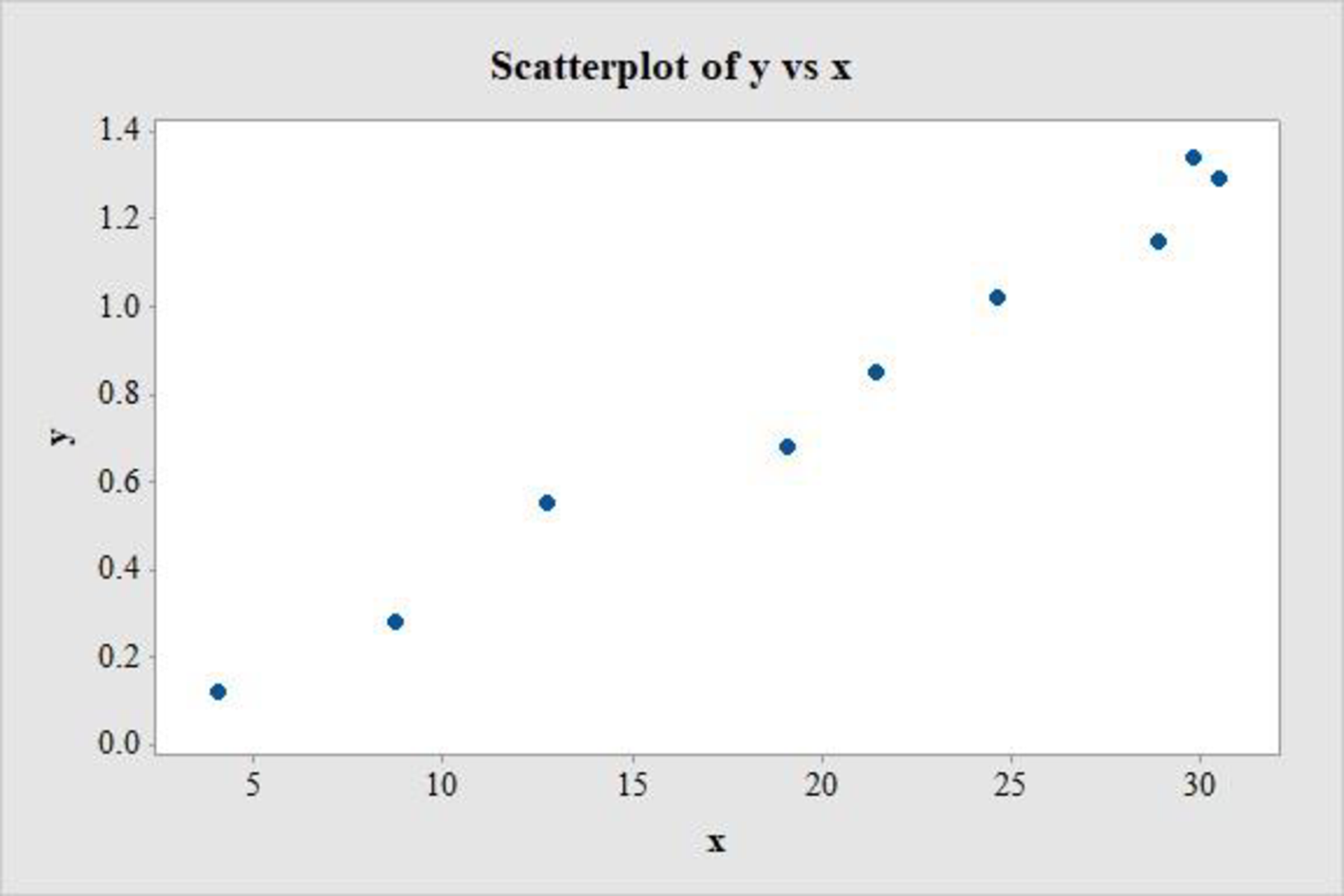
The scatter plot shows no apparent curve and there are no extreme observations. There is no change in the y values as the values of x change and there are no influential points. Therefore, the simple linear regression model seems appropriate for the data set.
b.
Find the equation of the estimated regression line by assuming that the simple linear regression model is appropriate.
Answer to Problem 60CR
The equation of the estimated regression line is,
Explanation of Solution
Calculation:
Regression Analysis:
Software procedure:
Step-by-step procedure to obtain the regression line using MINITAB software:
- Choose Stat > Regression > Regression > Fit Regression Model.
- Under Responses, enter the column of values y.
- Under Continuous predictors, enter the column of values x.
- Click OK.
Output using MINITAB software is given below:
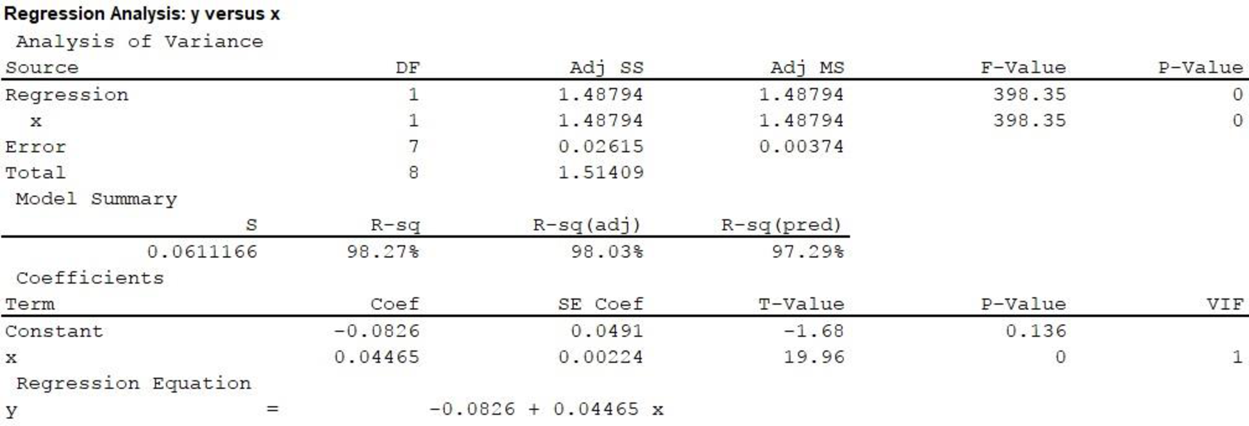
Hence, the equation of the estimated regression line by assuming that the simple linear regression model is appropriate is,
c.
Find how much of the observed variation in peak photo voltage can be explained by the model relationship.
Answer to Problem 60CR
The percentage of observed variation in peak photo voltage that can be explained by the model relationship is 98.3%.
Explanation of Solution
From the Minitab output in Part (b), the value of
This implies that 98.27%, or approximately 98.3% of the observed variation in the dependent variable ‘peak photo voltage’ is being explained by the independent variable ‘percentage of light absorption’ using the simple linear regression model. The change is attributable to the linear relationship between the variables ‘peak photo voltage’ and ‘percentage of light absorption’ and is being explained by the model.
Thus, the percentage of observed variation in peak photo voltage that can be explained by the model relationship is 98.3%.
d.
Predict peak photo voltage when percent absorption is 19.1.
Find the value of the corresponding residual.
Answer to Problem 60CR
The peak voltage when percent absorption is 19.1 is predicted to be 0.770.
The corresponding residual is –0.090.
Explanation of Solution
Calculation:
Predicted value:
The estimated regression equation is,
Hence, the peak voltage when percent absorption is 19.1 is predicted to be 0.770.
Residual:
The formula for residual for response, y and predicted response,
It is given that, when the percentage of light absorption is 19.1, the peak photo voltage is 0.68. Substitute
Hence, the corresponding residual is –0.09.
e.
Explain whether one can agree with the statement that there is a useful linear relationship between the two variables, by carrying out a formal test.
Explanation of Solution
Calculation:
1.
Here,
2.
Null hypothesis:
That is, there is no useful linear relationship between the percentage of light absorption and peak photo voltage.
3.
Alternative hypothesis:
That is, there is a useful linear relationship between the percentage of light absorption and peak photo voltage.
4.
Here, the significance level is assumed to be
5.
Test Statistic:
The formula for test statistic is as follows:
In the formula, b denotes the estimated slope,
6.
Assumption:
The assumption made in Part (b) is that, the simple linear regression model is appropriate.
7.
Calculation:
From the MINITAB output in Part (b), the t-test statistic value for
8.
P-value:
From the MINITAB output in Part (b), the P-value is 0.
9.
Decision rule:
- If P-value is less than or equal to the level of significance, reject the null hypothesis.
- Otherwise, fail to reject the null hypothesis.
10.
Conclusion:
The P-value is 0.
The level of significance is 0.05.
The P-value is less than the level of significance.
That is,
Based on rejection rule, reject the null hypothesis.
Thus, there is convincing evidence of a useful relationship between the percentage of light absorption and peak photo voltage at the 0.05 level of significance.
f.
Obtain an estimate of the average change in peak photo voltage associated with a 1 percentage point increase in light absorption.
Answer to Problem 60CR
The estimate of the average change in peak photo voltage associated with a 1 percentage point increase in light absorption is between 0.039 and 0.050.
Explanation of Solution
Calculation:
From the MINITAB output in Part (b), the value of slope is approximately
Formula for Degrees of freedom:
The formula for degrees of freedom is,
In the formula, n is the total number of observations.
Formula for Confidence interval for
In the formula b denotes the estimated slope and
Degrees of freedom:
The number of data values given are 9, that is
From the Appendix: Table 3 t Critical Values:
- Locate the value 7 in the degrees of freedom (df) column.
- Locate the 0.95 in the row of central area captured.
- The intersecting value that corresponds to the df 7 with confidence level 0.95 is 2.37.
Thus, the critical value for
Confidence interval:
Substitute,
Hence, the 95% confidence interval for estimating the average change in peak photo voltage associated with a 1 percentage point increase in light absorption is
Interpretation:
The 95% confidence interval can be interpreted as: there is 95% confidence that the mean increase in peak photo voltage associated with a 1 percentage point increase in light absorption lies between 0.039 and 0.050.
g.
Obtain an estimate of the average change in peak photo voltage when the percentage of light absorption is 20.
Answer to Problem 60CR
The estimate of the average change in peak photo voltage when the percentage of light absorption is 20 is between 0.762 and 0.859.
Explanation of Solution
Calculation:
The confidence interval for
From the MINITAB output in part (a), the simple linear regression model is
Point estimate:
The point estimate when the percentage of light absorption is 20 is calculated as follows.
Estimated standard deviation:
For the given x values,
Substitute,
Therefore, one can be 95% confident that the mean peak voltage when the percentage of light absorption is 20 is between 0.762 and 0.859.
Want to see more full solutions like this?
Chapter 13 Solutions
Introduction To Statistics And Data Analysis


- A U.S. state's Bureau of Economic Geology published a study on the economic impact of using carbon dioxide enhanced oil recovery (EOR) technology to extract additional oil from fields that have reached the end of their conventional economic life. The following table gives the approximate number of jobs for the citizens that would be created at various levels of recovery. Percent Recovery (%) 20 40 80 100 Jobs Created (Millions) 6 9 12 18 Find the regression line. j(r) = Use the regression line to estimate the number of jobs that would be created at a recovery level of 60%. _____ million jobsarrow_forwardAn econometrician suspects that the residuals of her model might be autocorrelated. Explain the steps involved in testing this theory using the Durbin–Watson (DW) testarrow_forwardThe table contains data on vehicle speed (h) and fuel consumption (lt / 100km) of 5 randomly selected vehicles. Estimate the average fuel consumption of a vehicle traveling at 45 km / h using the simple linear regression equation between vehicle speed and fuel consumption. Speed 55 60 65 70 75 Consumption 13 12 11 10 9 a. 15 b. 8 c. 7 d. 20arrow_forward
- In a laboratory experiment, data were gathered on the life span (y in months) of 33 rats, units of daily protein intake (x1), and whether or not agent x2 (a proposed life-extending agent) was added to the rats' diet (x2 = 0 if agent x2 was not added, and x2 = 1 if agent was added). From the results of the experiment, the following regression model was developed:ŷ = 36 + .8x1 − 1.7x2Also provided are SSR = 60 and SST = 180.The test statistic for testing the significance of the model is _____. a. 5.00 b. .50 c. .25 d. .33arrow_forwardThe following data is representative of that reported in an article on nitrogen emissions, with x = burner area liberation rate (MBtu/hr-ft2) and y = NOx emission rate (ppm): x 100 125 125 150 150 200 200 250 250 300 300 350 400 400 y 160 140 190 210 200 320 280 400 440 430 400 600 600 660 (a) Assuming that the simple linear regression model is valid, obtain the least squares estimate of the true regression line. (Round all numerical values to four decimal places.)y = (b) What is the estimate of expected NOx emission rate when burner area liberation rate equals 240? (Round your answer to two decimal places.)ppm(c) Estimate the amount by which you expect NOx emission rate to change when burner area liberation rate is decreased by 60. (Round your answer to two decimal places.)ppm(d) Would you use the estimated regression line to predict emission rate for a liberation rate of 500? Why or why not? Yes, the data is perfectly linear, thus lending to accurate predictions.…arrow_forwardA sixth-grade teacher believes that there is a relationship between his students’ IQscores (y) and the numbers of hours (x) they spend watching television each week. Thefollowing table shows a random sample of 7 sixth-grade students.y 125 116 97 114 85 107 105x 5 10 30 16 41 28 21 Does the data provide sufficient evidence to indicate that the simple linear regressionmodel is appropriate to describe the relationship between x and y? Perform a model utilitytest at α = 0.05. (Give H0, Ha, rejection region, observed test statistic, P-value, decisionand conclusion.)Find the Pearson sample correlation coefficient between x and y. Then interpretthe result.arrow_forward
- The table contains data on vehicle speed (h) and fuel consumption (lt / 100km) of 5 randomly selected vehicles. Estimate the average fuel consumption of a vehicle traveling at 45 km / h using the simple linear regression equation between vehicle speed and fuel consumption. Speed 55 60 65 70 75 Consumption 11 10 9 8 7 Please choose one: a. 6 b. 5 c. 13 D. 8arrow_forwardThe following table shows the annual number of PhD graduates in a country in various fields. NaturalSciences Engineering SocialSciences Education 1990 70 10 70 30 1995 130 40 110 40 2000 330 130 280 120 2005 490 370 460 210 2010 590 550 830 520 2012 690 590 1,000 900 (a) With x = the number of social science doctorates and y = the number of education doctorates, use technology to obtain the regression equation. (Round coefficients to three significant digits.) y(x) = (b) Use technology to obtain the coefficient of correlation r. (Round your answer to three decimal places.) r =arrow_forwardThe following are data on the average weekly profits(in $1,000) of five restaurants, their seating capacities, andthe average daily traffic (in thousands of cars) that passestheir locations: Seating Traffic Weekly netcapacity count profitx1 x2 y120 19 23.8200 8 24.2150 12 22.0180 15 26.2240 16 33.5 (a) Assuming that the regression is linear, estimate β0, β1,and β2.(b) Use the results of part (a) to predict the averageweekly net profit of a restaurant with a seating capacityof 210 at a location where the daily traffic count averages14,000 cars.arrow_forward
- The following table shows the annual number of PhD graduates in a country in various fields. NaturalSciences Engineering SocialSciences Education 1990 70 10 60 30 1995 130 40 120 50 2000 330 130 280 140 2005 490 370 460 210 2010 590 550 830 520 2012 690 590 1,000 900 (a) With x = the number of social science doctorates and y = the number of education doctorates, use technology to obtain the regression equation. (Round coefficients to three significant digits.) y(x) = Graph the associated points and regression line. (b) What does the slope tell you about the relationship between the number of social science doctorates and the number of education doctorates? The slope tells us the increase in the number of education doctorates for each additional social science doctorate.The slope tells us the decrease in the number of education doctorates for each additional social science doctorate. The slope tells us the increase in the number…arrow_forwardIn a certain type of metal test specimen, the normal stress on a specimen is known tobe functionally related to the shear resistance. The following is a set of codedexperimental data on the two variables:Normal stress (X) 26.8 25.4 28.9 23.6 27.7 23.9 24.7Shear resistance (Y) 26.5 27.3 24.2 27.1 23.6 25.9 26.3i) Estimate the linear regression line and interpret regressioncoefficient.ii) Comment about of goodness of fit of the estimated regression line.arrow_forwardThe following table shows the annual number of PhD graduates in a country in various fields. NaturalSciences Engineering SocialSciences Education 1990 70 10 70 30 1995 130 40 110 50 2000 330 130 280 140 2005 490 370 460 210 2010 590 550 830 520 2012 690 590 1,000 900 (a) With x = the number of social science doctorates and y = the number of education doctorates, use technology to obtain the regression equation. (Round coefficients to three significant digits.) y(x) = Graph the associated points and regression line. (b) What does the slope tell you about the relationship between the number of social science doctorates and the number of education doctorates? The slope tells us the increase in the number of social science doctorates for each additional education doctorate.The slope tells us the increase in the number of education doctorates for each additional social science doctorate. The slope tells us the decrease in the number…arrow_forward
 MATLAB: An Introduction with ApplicationsStatisticsISBN:9781119256830Author:Amos GilatPublisher:John Wiley & Sons Inc
 Probability and Statistics for Engineering and th...StatisticsISBN:9781305251809Author:Jay L. DevorePublisher:Cengage Learning
 Statistics for The Behavioral Sciences (MindTap C...StatisticsISBN:9781305504912Author:Frederick J Gravetter, Larry B. WallnauPublisher:Cengage Learning
 Elementary Statistics: Picturing the World (7th E...StatisticsISBN:9780134683416Author:Ron Larson, Betsy FarberPublisher:PEARSON
 The Basic Practice of StatisticsStatisticsISBN:9781319042578Author:David S. Moore, William I. Notz, Michael A. FlignerPublisher:W. H. Freeman
 Introduction to the Practice of StatisticsStatisticsISBN:9781319013387Author:David S. Moore, George P. McCabe, Bruce A. CraigPublisher:W. H. Freeman