
Videos
The article “Ultimate Load Analysis of Plate Reinforced Concrete Beams” (N. Subedi and P. Baglin, Engineering Structures, 2001:1068–1079) presents theoretical and measured ultimate strengths (in kN) for a sample of steel-reinforced concrete beams. The results are presented in the following table (two outliers have been deleted).
Let y denote the measured strength, x the theoretical strength, and t the true strength, which is unknown. Assume that y = t + ε, where ε is the measurement error. It is uncertain whether t is related to x by a linear model t = β0 + β1x or by a quadratic model t = β0 + β1x + β2x2.
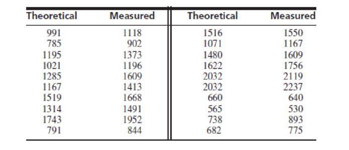
- a. Fit the linear model y = β0 + β1x + ε. For each coefficient, find the P-value for the null hypothesis that the coefficient is equal to 0.
- b. Fit the quadratic model y = β0 + β1x + β2x2 + ε. For each coefficient, find the P-value for the null hypothesis that the coefficient is equal to 0.
- c. Plot the residuals versus the lilted values for the linear model.
- d. Plot the residuals versus the fitted values for the quadratic model.
- e. c. Based on the results in parts (a) through (d), which model seems more appropriate? Explain.
- f. Using the more appropriate model, estimate the true strength if the theoretical strength is 1500.
- g. Using the mom appropriate model, find a 95% confidence interval for the true strength if the theoretical strength is 1500.
Want to see the full answer?
Check out a sample textbook solution
Chapter 8 Solutions
Statistics for Engineers and Scientists
Additional Math Textbook Solutions
Intro Stats, Books a la Carte Edition (5th Edition)
Essential Statistics
Elementary Statistics Using Excel (6th Edition)
EBK STATISTICAL TECHNIQUES IN BUSINESS
Business Analytics
Statistics: Informed Decisions Using Data (5th Edition)


- The article “Ultimate Load Analysis of Plate Reinforced Concrete Beams” (N. Subedi and P. Baglin, Engineering Structures, 2001:1068–1079) presents theoretical and measured ultimate strengths (in kN) for a sample of steel reinforced concrete beams. The results are presented in the following table (two outliers have been deleted). Let y denote the measured strength, x the theoretical strength, and t the true strength, which is unknown. Assume that y = t + ε, where ε is the measurement error. It is uncertain whether t is related to x by a linear model t = β0 + β1x or by a quadratic model t = β0 + β1x + β2x2. Fit the quadratic model y = β0 + β1x + β2x2 + ε. For each coefficient, find the P-value for the null hypothesis that the coefficient is equal to 0. a) Since (Click to select one) P < 0.001 , 0.001 < P < 0.002 , 0.002 < P < 0.01 , 0.01 < P < 0.02 , 0.02 < P < 0.05 , 0.05 < P < 0.10 , 0.10 < P < 0.20 , 0.20 < P < 0.50 , 0.50 <…arrow_forwardQ1 A) List down the measures of central tendency and measures of dispersion 2) The operations manager of a plant that manufactures tires wants to compare the actual inner diameters of two grades of tires, each of B) which is expected to be 575 millimeters. A sample of five tires of each grade was selected, and the results representing the inner diameters of the tires, ranked from smallest to largest, are as follows. Grade X grade Y 568 570 575 578 584 573 574 575 577 578 requirement. a) for each of the tow grades of tries, compute the mwan, median, and standred deviation. b) which grade of tire providing better quality? explain. c) what would be the effect on your answer in (a) and (b) if the last value for grade Y were 588 insert 578 explain. C) The file contins the overall miles per gallon (MPG) OF 2010 family sedan: 24 21 22 23 24 34 34 34 20 20 22 22 44 32 20 20 22 20 39 20 Source:…arrow_forwardFoot ulcers are a common problem for people with diabetes. Higher skin temperatures on the foot indicate an increased risk of ulcers. The article "An Intelligent Insole for Diabetic Patients with the Loss of Protective Sensation" (Kimberly Anderson, M.S. Thesis, Colorado School of Mines), reports measurements of temperatures, in °F, of both feet for 181 diabetic patients. The results are presented in the following table. Left Foot Right Foot 80 80 85 85 75 80 88 86 89 87 87 82 78 78 88 89 89 90 76 81 89 86 87 82 78 78 80 81 87 82 86 85 76 80 88 89 Construct a scatterplot of the right foot temperature (y) versus the left foot temperature (x). Verify that a linear model is appropriate. b. Compute the least-squares line for predicting the right foot temperature from the left foot temperature. If the left foot temperatures of two patients differ by 2 degrees, by how much would you predict their right foot temperatures to differ? Predict the right foot temperature for a patient whose left…arrow_forward
- Following are measurements of soil concentrations (in mg /kg) of chromium (Cr) and nickel (Ni) at20 sites in the area of Cleveland, Ohio. These data are taken from the article "Variation in NorthAmerican Regulatory Guidance for Heavy Metal Surface Soil Contamination at Commercial andIndustrial Sites" (A. Jennings and J. Ma, J. Environment Eng, 2007:587-609).Cr: 260 19 36 247 263 319 317 277 319 264 23 29 61 119 33 281 21 35 64 30Ni: 435 377 359 53 38 38 54 188 397 33 92 490 28 35 799 347 321 32 74 508 (d) Use these to construct comparative boxplots for the two sets of concentrations. (e) Using the boxplots, what differences can be seen between the two sets of concentrations?arrow_forwardThe article "Modeling Resilient Modulus and Temperature Correction for Saudi Roads" (H. Wahhab, I. Asi, and R. Ramadhan, Journal of Materials in Civil Engineering, 2001:298– 305) describes a study designed to predict the resilient modulus of pavement from physical properties. The following table presents data for the resilient modulus at 40°Cin10® kPa (y), the surface area of the aggregate in m²/kg (x1), and the softening point of the asphalt in °C (х). y X1 X2 1.48 5.77 60.5 1.70 7.45 74.2 2.03 8.14 67.6 2.86 8.73 70.0 2.43 7.12 64.6 3.06 6.89 65.3 2.44 8.64 66.2 1.29 6.58 64.1 3.53 9.10 68.6 1.04 8.06 58.8 1.88 5.93 63.2 1.90 8.17 62.1 1.76 9.84 68.9 2.82 7.17 72.2 1.00 7.78 54.1 The full quadratic model is y = + P,x, + PzX, + Pz*jXz + Pxx¡ + Bzx; + €. Which submodel of this full model do you believe is most appropriate? Justify your answer by fitting two or more models and comparing the results.arrow_forwardThe spike stature of the plants grown from the seeds of the porcine separates (Dactylis glomerata L) collected from the University campus and İbradı Eynif pasture are given below. In this plant, compare whether there is a difference between regions in terms of spike height. Virgo Height (cm) Data obtained from plants collected from university campus 5 6 8 7 8 6 5 5 4 6 6 Data obtained from plants collected from Eynif pasture 12 9 11 9 9 11 9 10 11 10 Note: Your results interpretation according to two different possibilities (Do it separately, assuming that it is 0.07 and 0.04).arrow_forward
- 1. Analyze the data as a two way factorial design. Johnson and Leone (Statistics and Experimental Design in Engineering and the Physical Sciences, Wiley, 977) describe an experiment to investigate warping of copper plates. The two factors studied were the temperature and the copper content of the plates. The response variable was a measure of the amount of warping. The data were as follows: Temperature (°C) 50 75 100 125 40 17, 20 12,9 16, 12 21, 17 Copper Content (%) 60 80 16, 21 18, 13 18, 21 23, 2! 24, 22 17, 12 25, 23 23, 22 100 28, 27 27, 31 30, 23 29, 31arrow_forwardA study was conducted in the tidal flat at Polka Point, North Stradbroke Island to examine the distribution of the animals that live with the seagrass Sargassum at different distances from the shoreline. Samples of Sargassum were taken at 5, 10, 15 m from the shore and these were examined for amphipods and isopods. The observations are recorded below. Is the distribution of each of the organisms with regards to the shore the same at all three distances? Use the data below to test the hypothesis at the p < 0.05 level. Clearly state the hypotheses and interpret the results. (Note: Find chi-square for each individual column (amphipods and isopods, not the two together) Distance Amphipods Isopods 5 2 7 10 31 14 15 45 22arrow_forwardAn article in the Fire Safety Journal (“The Effect of Nozzle Design on the Stability and Performance of Turbulent Water Jets,” Vol. 4, August 1981) describes an experiment in which a shape factor was determined for several different nozzle designs at six levels of jet efflux velocity. Interest focused on potential differences between nozzle designs (blocks), with velocity considered as a nuisance variable. The data are shown below: Jet Efflux Velocity (m/s) Nozzle Design 11.73 14.37 16.59 20.43 23.46 28.74 1 0.78 0.80 0.81 0.75 0.77 0.78 2 0.85 0.85 0.92 0.86 0.81 0.83 3 0.93 0.92 0.95 0.89 0.89 0.83 4 1.14 0.97 0.98 0.88 0.86 0.83 5 0.97 0.86 0.78 0.76 0.76 0.75 1) Write the null hypothesis and the alternative hypothesis (for the factor). 2) Find the ANOVA table. (round to five decimal places). 3) What is your decision about the null hypothesis, consider ?. 4) If your decision in part (4) was reject , perform Tukey test to determine which pairwise means are…arrow_forward
- The article in the ASCE Journal of Energy Engineering (1999, Vol. 125, pp.59-75) describes a study of the thermal inertia properties of autoclaved aerated concrete used as a building material. Five samples of the material were tested in a structure, and the average interior temperatures (°C) reported were as follows: 23.01, 22.22, 22.04, 22.62, and 22.59. Test that the average interior temperature is equal to 22.5°C using alpha (a) = 0.05. This problem is a test on what population parameter? What is the null and alternative hypothesis? What are the Significance level and type of test? What standardized test statistic will be used? What is the standard test statistic? What is the Statistical Decision? What is the statistical decision in the statement form?arrow_forwardSnow avalanches can be a real problem for travelers in the western United States and Canada. A very common type of avalanche is called the slab avalanche. These have been studied extensively by David McClung, a professor of civil engineering at the University of British Columbia. Suppose slab avalanches studied in a region of Canada had an average thickness of u = 67 cm. The ski patrol at Vail, Colorado, is studying slab avalanches in its region. A random sample of avalanches in spring gave the following thicknesses (in cm). 59 51 76 38 65 54 49 62 68 55 64 67 63 74 65 79 (i) Use a calculator with sample mean and standard deviation keys to find x and s. (Round your answers to two decimal places.) X= cm S= cm (ii) Assume the slab thickness has an approximately normal distribution. Use a 1% level of significance to test the claim that the mean slab thickness in the Vail region is different from that in the region of Canada. (a) What is the level of significance? State the null and…arrow_forwardA) In the screenshot i provided B) Does either explanatory variable improve the fit of the model that uses the other? Use a test statistic for each. Use α=0.05.arrow_forward
 Linear Algebra: A Modern IntroductionAlgebraISBN:9781285463247Author:David PoolePublisher:Cengage Learning
 Calculus For The Life SciencesCalculusISBN:9780321964038Author:GREENWELL, Raymond N., RITCHEY, Nathan P., Lial, Margaret L.Publisher:Pearson Addison Wesley,
 Glencoe Algebra 1, Student Edition, 9780079039897...AlgebraISBN:9780079039897Author:CarterPublisher:McGraw Hill