
Videos
(Continues Exercise 7 in Section 8.1.) To try to improve the prediction of FEV1, additional independent variables are included in the model. These new variables are Weight (in kg), the product (interaction) of Height and Weight, and the ambient temperature (in °C). The following MINITAB output presents results of fitting the model
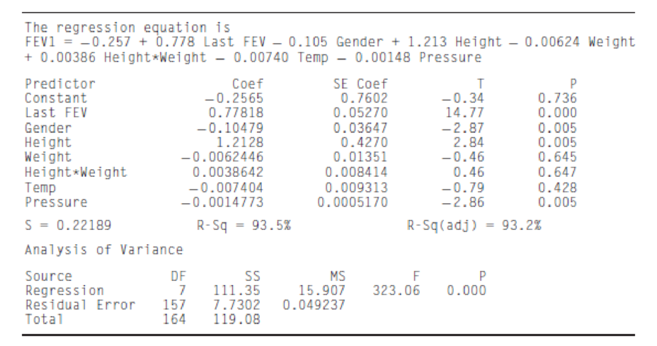
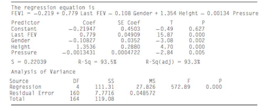
- a. The following MINITAB output, reproduced from Exercise 7 in Section 8.1, is for a reduced model in which Weight, Height·Weight, and Temp have been dropped. Compute the F statistic for testing the plausibility of the reduced model.
- b. How many degrees of freedom does the F statistic have?
- c. Find the P-value for the F statistic. Is the reduced model plausible?
- d. Someone claims that since each of the variables being dropped had large P-values, the reduced model must be plausible, and it was not necessary to perform an F test. Is this correct? Explain why or why not.
Want to see the full answer?
Check out a sample textbook solution
Chapter 8 Solutions
Statistics for Engineers and Scientists
Additional Math Textbook Solutions
Essentials of Statistics (6th Edition)
Fundamentals of Statistics (5th Edition)
Statistics for Business & Economics, Revised (MindTap Course List)
Introduction to Statistical Quality Control
Statistical Techniques in Business and Economics


- The least-squares regression equation is y=620.6x+16,624 where y is the median income and x is the percentage of 25 years and older with at least a bachelor's degree in the region. The scatter diagram indicates a linear relation between the two variables with a correlation coefficient of 0.7004. In a particular region, 28.3 percent of adults 25 years and older have at least a bachelor's degree. The median income in this region is $37,389. Is this income higher than what you would expect? Why?arrow_forwardConsider the one-variable regression model Yi = β0 + β1Xi + ui, and suppose it satisfies the least squares assumptions in Key Concept 4.3. Suppose Yi is measured with error, so the data are ?"i = Yi + wi, where wi is the measurement error, which is i.i.d. and independent of Yi. Consider the population regression ?"i = β0 + β1Xi + vi, where vi is the regression error, using the mismeasured dependent variable ?"i.a) Showthatvi =ui +wi.b) Show that the regression ?"i = β0 + β1Xi + vi satisfies the least squares assumptions in KeyConcept 4.3. (Assume that wi is independent of Yj and Xj for all values of i and j and has afinite fourth moment.)c) Are the OLS estimators consistent? part b in another questionarrow_forwardA researcher wishes to build an appropriate multiple linear model for predicting response variable Y using three predictor variables X1, X2, and X3. He has just made sixteen observations and analysed his data using SPSS. Part of his analysis outputs is as given in the table below. Unstandardized Standardized Coefficients Coefficients Model B Std. Error Beta (Constant) 33.964 13.061 X1 2.960 1.227 .519 X2 .702 .946 .140 X3 -1.769 .702 -.343 2.1 Interpret the unstandardized coefficient of X3. 2.2 Construct the ANOVA table for his model given that SSR = 8417.884 and that MSE = 6.843. 2.3 Compute the adjusted R square for this model and interpret it. 2.4 Compute observed t-values for all model parameters. 2.5 Construct the 95% confidence intervals for all slope parameters and hence use them to determine all significant predictors of Y, if any, at 5% level?arrow_forward
- In a statistical study, it is found that variables x and y are correlated as follows. Find the least squares regression line in this model.arrow_forwardA medical researcher conducted an observational study to understand the recovery rate for patients infected with the COVID-19 in Malaysia. The researcher contacted thirteen COVID-19 survivors and interviewed them regarding their recovery experience. Two of the questions asked are the recovery period (in days) and the number of days that have passed since receiving the second dose of COVID-19 vaccine prior to infection. The recorded data is summarized as (at the image files). i) Identify the dependent variable in the study. ii) Calculate the correlation coefficient and interpret its value. iii) Estimate the regression model parameters and write the estimated linear regression model. iv) Based on your answer in iii), predict the recovery period if a person is infected with COVID-19 after 200 days of receiving second dose of COVID-19 vaccine. v) Table 1 represents the incomplete ANOVA table of the study. Find the values of P, Q, R and S. vi) Test the linearity between the two variables…arrow_forwardThe least-squares regression equation is y=784.6x+12,431 where y is the median income and x is the percentage of 25 years and older with at least a bachelor's degree in the region. The scatter diagram indicates a linear relation between the two variables with a correlation coefficient of 0.7962. In a particular region, 26.5 percent of adults 25 years and older have at least a bachelor's degree. The median income in this region is $29,889. Is this income higher or lower than what you would expect? Why?arrow_forward
- A random sample of 65 high school seniors was selected from all high school seniors at a certain high school. A scatterplot (not shown) revealed the height, in cm and foot length in cm, for each high school student from the sample. The association was described to be strong, positive, and linear. a. In the context of the study, explain what is meant by the following terms: positive: linear: b. The least squares regression equation was predicted height=105.08+2.599 (foot length). One of the students had a foot length of 20 cm. His residual was calculated to be 2.94 cm. What was the height of the student? c. suppose that the distribution of residuals is approximately normal with a standard deviation of 5.9 cm. What percent of residuals are less than 7 cm? Justify why.arrow_forwardThe least-squares regression equation is y=620.6x+16,624 where y is the median income and x is the percentage of 25 years and older with at least a bachelor's degree in the region. The scatter diagram indicates a linear relation between the two variables with a correlation coefficient of 0.7004. Predict the median income of a region in which 30% of adults 25 years and older have at least a bachelor's degree.arrow_forwardtion 13 A least squares regression line a. may be used to predict a value of y if the corresponding value is given O b. implies a cause-effect relationship between x and y O c. can only be determined if a good linear relationship exists between x and y Od. All of these answers are correct.arrow_forward
- Dr. Rancur believes that working memory errors (M) will increase linearly with increases in level of cognitive load (CL). He randomly assigns 10 subjects to each of four cognitive load levels: 1, 3, 5 and 7 and assesses subjects’ memory performance. The results of his study are exhaustively summarized below. Using the summary information, carry out an analysis to determine if M is related to CL in the way Dr. Rancur predicts. Make sure you estimate the magnitude of the association, and construct a confidence interval as appropriate. In a summary sentence or two, evaluate the evidence for or against Dr. Rancur’s prediction.arrow_forwardAn aircraft company wanted to predict the number of worker-hours necessary to finish the design of a new plane. Relevant explanatory variables were thought to be the plane’s top speed, its weight, and the number of parts it had in common with other models built by the company. A sample of 27 of the company’s planes was taken, and the following model was estimated: y = 0 +11+22+33+ Where y = design effort, in millions of worker-hours 1 = plane’s top speed, in miles per hour 2= plane’s weight, in tons 3 = percentage of parts in common with other models The estimated regression coefficients were as follows: b1 = 0.661 b2 = 0.065 b3 = - 0.018 The total sum of squares and regression sum of squares were found to be as follows: SST = 3.881 and SSR = 3.549 Compute and interpret the coefficient of determination. Compute the error sum of squares. Compute the adjusted coefficient of determination. Compute and interpret the coefficient of multiple correlation.arrow_forwardIn the context of a controlled experiment, consider the simple linear regression formulation Yi = β0 + β1Xi + Ui. Let the Yi be the outcome, Xi the treatment level when the treatment is binary, and Ui contain all the additional determinants of the outcome. Then: a. the OLS estimator of the slope will be inconsistent in the case of a randomly assigned Xi since there are omitted variables present. b. Xi and Ui will not be independently distributed if the Xi are randomly assigned. c. β0 represents the causal effect of X on Y when X is zero. d. E(Y|X= 1) is the expected value for the treatment group. e. All of the above. f. None of the above.arrow_forward
 Calculus For The Life SciencesCalculusISBN:9780321964038Author:GREENWELL, Raymond N., RITCHEY, Nathan P., Lial, Margaret L.Publisher:Pearson Addison Wesley,
 Linear Algebra: A Modern IntroductionAlgebraISBN:9781285463247Author:David PoolePublisher:Cengage Learning