
Concept explainers
Videos
The article “Change in Creep Behavior of Plexiform Bone with Phosphate Ion Treatment” (R. Regimbal, C. DePaula, and N. Guzelsu, Bio-Medical Materials and Engineering, 2003:11–25) describes an experiment to study the effects of saline and phosphate ion solutions on mechanical properties of plexiform bone. The following table presents the yield stress measurements for six specimens treated with cither saline (NaCl) or phosphate ion (Na2HPO4 ) solution, at a temperature of either 25°C or 37°C. (The article presents means and standard deviations only; the values in the table are consistent with these.)
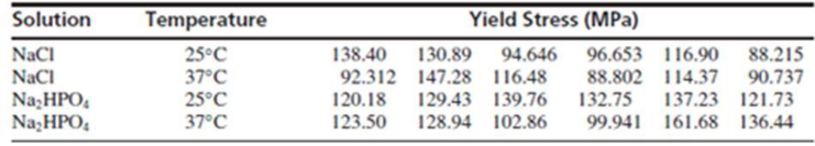
- a. Estimate all main effects and interactions.
- b. Construct an ANOVA table. You may give
ranges for the P-values. - c. Is the additive model plausible? Provide the value of the test statistic and the P-value.
- d. Can the effect of solution (NaCl versus Na2HPO4) on yield stress be described by interpreting the main effects of solution? If so, interpret the main effects, including the appropriate test statistic and P-value. If not, explain why not.
- e. Can the effect of temperature on yield stress be described by interpreting the main effects of temperature? If so, interpret the main effects, including the appropriate test statistic and P-value. If not, explain why not.
Want to see the full answer?
Check out a sample textbook solution
Chapter 9 Solutions
Statistics for Engineers and Scientists
Additional Math Textbook Solutions
Applied Statistics in Business and Economics
Stats: Modeling the World Nasta Edition Grades 9-12
Introductory Statistics
Basic Business Statistics, Student Value Edition
PRACTICE OF STATISTICS F/AP EXAM


- The depth of wetting of a soil is the depth to which water content will increase owing to extemal factors. The article "Discussion of Method for Evaluation of Depth of Wetting in Residential Areas" (J. Nelson, K. Chao, and D. Overton, Journal of Geotechnical and Geoenvironmental Engineering, 2011:293-296) discusses the relationship between depth of wetting beneath a structure and the age of the structure. The article presents measurements of depth of wetting, in meters, and the ages, in years, of 21 houses, as shown in the following table. Age Depth 7.6 4 4.6 6.1 9.1 3 4.3 7.3 5.2 10.4 15.5 5.8 10.7 4 5.5 6.1 10.7 10.4 4.6 7.0 6.1 14 16.8 10 9.1 8.8 Compute the least-squares line for predicting depth of wetting (y) from age (x). b. Identify a point with an unusually large x-value. Compute the least-squares line that results from deletion of this point. Identify another point which can be classified as an outlier. Compute the least-squares line that results from deletion of the outlier,…arrow_forwardThe article "Effect of Granular Subbase Thickness on Airfield Pavement Structural Response" (K. Gopalakrishnan and M. Thompson, Journal of Materials in Civil Engineering, 2008:331-342) presents a study of the amount of surface deflection caused by aircraft landing on an airport runway. A load of 160 kN was applied to a runway surface, and the amount of deflection in mm (y) was measured at various distances in m (x) from the point of application. The results are presented in the following table. y 0.000 3.24 0.305 2.36 0.610 1.42 0.914 0.87 1.219 0.54 1.524 0.34 1.830 0.24 a. Fit the linear model y = Bo + B1x + ɛ. For each coefficient, test the hypothesis that the coefficient is equal to 0. b. Fit the quadratic model y = Bo + Bịx + B2x² + ɛ. For each coefficient, test the hypothesis that the coefficient is equal to 0. %3D Fit the cubic model y = Bo + B1x + B2x? + B3x + E. For each coefficient, test the C. hypothesis that the coefficient is equal to 0. d. Which of the models in parts (a)…arrow_forwardThe article “Effect of Granular Subbase Thickness on Airfield Pavement Structural Response” (K. Gopalakrishnan and M. Thompson, Journal of Materials in Civil Engineering, 2008:331–342) presents a study of the effect of the subbase thickness on the amount of surface deflection caused by aircraft landing on an airport runway. In six applications of a 160 kN load on a runway with a subbase thickness of 864 mm, the average surface deflection was 2.03 mm with a standard deviation of 0.090 mm. Find a 90% confidence interval for the mean deflection caused by a 160 kN load.arrow_forward
- The article “Effect of Varying Solids Concentration and Organic Loading on the Performance of Temperature Phased Anaerobic Digestion Process” (S. Vandenburgh and T. Ellis, Water Environment Research, 2002:142–148) discusses experiments to determine the effect of the solids concentration on the performance of treatment methods for wastewater sludge. In the first experiment, the concentration of solids (in g/L) was 43.94 ± 1.18. In the second experiment, which was independent of the first, the concentration was 48.66 ± 1.76. Estimate the difference in the concentration between the two experiments, and find the uncertainty in the estimate.arrow_forwardThe article “Some Parameters of the Population Biology of Spotted Flounder (Ciutharuslinguatula Linnaeus, 1758) in Edremit Bay (North Aegean Sea)” (D. Türker, B. Bayhan, etal., Turkish Journal of Veterinary and Animal Science, 2005:1013–1018) models therelationship between weight W and length L of spotted flounder as W = aLb where a and bare constants to be estimated from data. Transform this equation to produce a linear model.arrow_forwardAdding glass particles to clay brick may improve the structural properties of the brick. The article "Effects of Waste Glass Additions on the Properties and Durability of Fired Clay Brick" (S. Chidiac and L. Federico, Can J Civ Eng, 2007:1458–1466) describes experiments in which the compressive strength (in MPa) was measured for bricks with varying amounts of glass content and glass particle size. The results in the following table are consistent with means and standard deviations presented in the article. Glass Content (%) Strength (MPa) Size 5 Coarse 78.7 70.8 78.6 81.7 79.2 5 Fine 73.0 90.1 71.4 93.8 82.7 10 Coarse 80.1 76.9 76.5 84.3 77.7 10 Fine 76.2 80.1 121.2 81.4 61.2 15 Coarse 90.3 95.8 103.1 99.5 73.3 15 Fine 141.1 144.1 122.4 134.5 124.9 a. Estimate all main effects and interactions. b. Construct an ANOVA table. You may give ranges for the P-values. Is the additive model plausible? Provide the value of a test statistic and the P-value. Can the effect of glass content on…arrow_forward
- Please show me your solutions and interpretations. Show the completehypothesis-testing procedure.An article in the ASCE Journal of Energy Engineering (1999, Vol. 125, pp. 59–75) describes a study of the thermal inertia properties of autoclaved aerated concrete used as a building material. Five samples of the material were tested in a structure, and the average interior temperatures (°C) reported were as follows: 23.01, 22.22, 22.04, 22.62, and 22.59. Test that the average interior temperature is equal to 22.5 °C using α = 0.05.arrow_forwardThe article "Effect of Refrigeration on the Potassium Bitartrate Stability and Composition of Italian Wines" (A. Versari, D. Barbanti, et al., Italian Journal of Food Science, 2002:45- 52) reports a study in which eight types of white wine had their tartaric acid concentration (in g/L) measured both before and after a cold stabilization process. The results are presented in the following table: Wine Type Before After Difference 2.86 2.59 0.27 2.85 2.47 0.38 3 1.84 1.58 0.26 4 1.60 1.56 0.04 0.80 0.78 0.02 6. 0.89 0.66 0.23 2.03 1.87 0.16 1.90 1.71 0.19 Find a 95% confidence interval for the mean difference between the tartaric acid concentrations before and after the cold stabilization process.arrow_forwardThe article "Effect of Granular Subbase Thickness on Airfield Pavement Structural Response" (K. Gopalakrishnan and M. Thompson, Journal of Materials in Civil Engineering, 2008:331-342) presents a study of the effect of the subbase thickness (in mm) on the amount of surface deflection caused by aircraft landing on an airport runway. Two landing gears, one simulating a Boeing 747 aircraft, and the other a Boeing 777 aircraft, were trafficked across four test sections of runway. The results are presented in the following table. Section 3 4 Boeing 747 Boeing 777 4.01 3.87 3.72 3.76 4.57 4.48 4.36 4.43 Can you conclude that the mean deflection is greater for the Boeing 777?arrow_forward
- The decline of salmon fisheries along the Columbia River in Oregon has caused great concern among commercial and recreational fishermen. The paper 'Feeding of Predaceous Fishes on Out-Migrating Juvenile Salmonids in John Day Reservoir, Columbia River' (Trans. Amer. Fisheries Soc. (1991: 405-420)) gave the accompanying data on y = maximum size of salmonids consumed by a northern squaw fish (the most abundant salmonid predator) and x = squawfish length, both in mm. Use the following statistics to give the equation of the least squares regression line.x = 524.800, y = 303.660, sx = 14.429, sy = 11.200, r = 0.9662 a) ŷ = 1.245x − 89.940 b) ŷ = 0.750x − 89.940 c) ŷ = -89.940x + 0.750 d) ŷ = 1.245x + 89.940 e) ŷ = 0.750x + 89.940 f) None of the abovearrow_forwardThe article "Characterization of Effects of Thermal Property of Aggregate on the Carbon Footprint of Asphalt Industries in China" (A. Jamshidi, K. Kkurumisawa, et al., Journal of Traffic and Transportation Engineering 2017: 118-130) presents the results measurements of CO, emissions produced during the manufacture of asphalt. Three measurements were taken at each of three mixing temperatures. The results are presented in the following table: Temperature (*C) Emissions (100kt) 160 9.52 14.10 7.43 145 8.37 6.54 12.40 130 7.24 10.70 5.66 Construct an ANOVA table. You may give a range for the P-value. Can you conclude that the mean emissions differ with mixing temperature? a.arrow_forwardThe article "Oxidation State and Activities of Chromium Oxides in Cao-SiO,-CrO, Slag System" (Y. Xiao, L. Holappa, and M. Reuter, Metallurgical and Materials Transactions B, 2002:595-603) presents the amount x (in mole percent) and activity coefficient y of CrO,5 for several specimens. The data, extracted from a larger table, are presented in the following table. х У 2.6 10.20 5.03 19.9 8.84 0.8 6.62 5.3 2.89 20.3 2.31 39.4 7.13 5.8 3.40 29.4 5.57 2.2 7.23 5.5 2.12 33.1 1.67 44.2 5.33 13.1 16.70 0.6 9.75 2.2 2.74 16.9 2.58 35.5 1.50 48.0 Compute the least-squares line for predicting y from x. b. Plot the residuals versus the fitted values. Compute the least-squares line for predicting y from 1/x. d. Plot the residuals versus the fitted values. C. Using the better fitting line, find a 95% confidence interval for the mean value of y when x= 5.0.arrow_forward
 MATLAB: An Introduction with ApplicationsStatisticsISBN:9781119256830Author:Amos GilatPublisher:John Wiley & Sons Inc
 Probability and Statistics for Engineering and th...StatisticsISBN:9781305251809Author:Jay L. DevorePublisher:Cengage Learning
 Statistics for The Behavioral Sciences (MindTap C...StatisticsISBN:9781305504912Author:Frederick J Gravetter, Larry B. WallnauPublisher:Cengage Learning
 Elementary Statistics: Picturing the World (7th E...StatisticsISBN:9780134683416Author:Ron Larson, Betsy FarberPublisher:PEARSON
 The Basic Practice of StatisticsStatisticsISBN:9781319042578Author:David S. Moore, William I. Notz, Michael A. FlignerPublisher:W. H. Freeman
 Introduction to the Practice of StatisticsStatisticsISBN:9781319013387Author:David S. Moore, George P. McCabe, Bruce A. CraigPublisher:W. H. Freeman