
Videos
The article “Cellulose Acetate Microspheres Prepared by O/W Emulsification and Solvent Evaporation Method” (K. Soppinmath, A Kulkarni, et al., Journal of Microncapsulation, 2001:811–817) describes a study of the effects of the concentrations of polyvinyl alcohol (PVAL) and dichloromethane (DCM) on the encapsulation efficiency in a process that produces microspheres containing the drug ibuprofen. There were three concentrations of PVAL (measured in units of % w/v) and three of DCM (in ml.). The results presented in the following table are consistent with the means and standard deviations presented in the article.
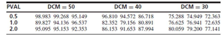
- a. Construct an ANOVA table. You may give
ranges for the P-values. - b. Discuss the relationships among PVAL concentration, DCM concentration, and encapsulation efficiency.
Want to see the full answer?
Check out a sample textbook solution
Chapter 9 Solutions
Statistics for Engineers and Scientists
Additional Math Textbook Solutions
Introductory Statistics (10th Edition)
Research Methods for the Behavioral Sciences (MindTap Course List)
Statistics for Business & Economics, Revised (MindTap Course List)
Elementary Statistics (Text Only)
Essentials of Statistics, Books a la Carte Edition (5th Edition)


- Acrylic resins used in the fabrication of dentures should not absorb much water, since water sorption reduces strength. The article "Reinforcement of Acıylic Resin for Provisional Fixed Restorations. Part III: Effects of Addition of Titania and Zirconia Mixtures on Some Mechanical and Physical Properties" (W. Panyayong, Y. Oshida, et al., Bio-Medical Materials and Engineering, 2002:353-366) describes a study of the effect on water sorption of adding titanium dioxide (TiO,) and zirconium dioxide (ZiO,) to a standard acıylic resin. Twelve specimens from each of several formulations, containing various amounts of TiO, and Zro, were immersed in water for one week, and the water sorption (in ug/mm?) was measured in each. The results are presented in the following table. Volume % Formulation TIO, Zro, Mean A (control) Standard Deviation 24.03 2.50 14.88 1.55 2 12.81 1.08 0.5 11.21 2.98 2 16.05 1.66 12.87 0.96 15.23 0.97 Н 3 15.37 0.64 Use the Bonferoni method to determine which of the…arrow_forwardFluid inclusions are microscopic volumes of fluid that are trapped in rock during rock formation. The article "Fluid Inclusion Study of Metamorphic Gold-Quartz Veins in Northwestern Nevada, U.S.A.: Characteristics of Tectonically Induced Fluid" (S. Cheong, Geosciences Journal, 2002:103-115) describes the geochemical properties of fluid inclusions in several different veins in northwest Nevada. The following table presents data on the maximum salinity (% NaCi by weight) of inclusions in several rock samples from several areas. Salinity Area Humboldt Range Santa Rosa Range 9.2 10.0 11.2 8.8 5.2 6.1 8.3 Ten Mile 7.9 6.7 9.5 7.3 10.4 7.0 Antelope Range Pine Forest Range 6.7 8.4 9.9 10.5 16.7 17.5 15.3 20.0 Can you conclude that the salinity differs among the areas?arrow_forwardIn "Orthogonal Design for Process Optimization and Its Application to Plasma Etching" (Solid State Technology, May 1987), G. Z. Yin and D. W. Jillie describe an experiment to determine the effect of C2Fe flow rate on the uniformity of the etch on a silicon wafer used in integrated circuit manufacturing. Three flow rates are used in the experiment, and the resulting uniformity (in percent) for six replicates is shown below. Observations C„F. Flow (SCCM) 2 3 4 5 125 2.5 4.4 2.6 3.2 3.2 4.0 160 4.8 4.4 4.8 4.2 3.6 4.2 200 4.6 3.3 2.8 3.4 4.2 5.3 (a) Does C,F, flow rate affect etch uniformity? Construct box plots to compare the factor levels and perform the analysis of variance. Use a = 0.05. There is that flow rate affects etch uniformity. (b) Do the residuals indicate any problems with the underlying assumptions? No. Statistical Tables and Charts Yes.arrow_forward
- The article "Influence of Freezing Temperature on Hydraulic Conductivity of Silty Clay" (J. Konrad and M. Samson, Journal of Geotechnical and Geoenvironmental Engineering, 2000:180–187) describes a study of factors affecting hydraulic conductivity of soils. The measurements of hydraulic conductivity in units of 108 cm/s (y), initial void ratio (x), and thawed void ratio (x2) for 12 specimens of silty clay are presented in the following table. y 1.01 1.12 1.04 1.30 1.01 1.04 0.955 1.15 1.23 1.28 1.23 1.30 0.84 0.88 0.85 0.95 0.88 0.86 0.85 0.89 0.90 0.94 0.88 0.90 X1 0.81 0.85 0.87 0.92 0.84 0.85 0.85 0.86 0.85 0.92 0.88 0.92 X2 Fit the model y = Bo + fix1 + e. For each coefficient, test the null hypothesis that it is equal to 0. Fit the model y = Bo + Bzx2 + e. For each coefficient, test the null hypothesis that it is equal to 0. Fit the model y = Bo + BzX1 + Bzxz + e. For each coefficient, test the null hypothesis that it is equal to 0. d. Which of the models in parts (a) to (c) is…arrow_forwardThe article "Effect of Granular Subbase Thickness on Airfield Pavement Structural Response" (K. Gopalakrishnan and M. Thompson, Journal of Materials in Civil Engineering, 2008:331-342) presents a study of the amount of surface deflection caused by aircraft landing on an airport runway. A load of 160 kN was applied to a runway surface, and the amount of deflection in mm (y) was measured at various distances in m (x) from the point of application. The results are presented in the following table. y 0.000 3.24 0.305 2.36 0.610 1.42 0.914 0.87 1.219 0.54 1.524 0.34 1.830 0.24 a. Fit the linear model y = Bo + B1x + ɛ. For each coefficient, test the hypothesis that the coefficient is equal to 0. b. Fit the quadratic model y = Bo + Bịx + B2x² + ɛ. For each coefficient, test the hypothesis that the coefficient is equal to 0. %3D Fit the cubic model y = Bo + B1x + B2x? + B3x + E. For each coefficient, test the C. hypothesis that the coefficient is equal to 0. d. Which of the models in parts (a)…arrow_forwardThe article "Experimental Measurement of Radiative Heat Transfer in Gas-Solid Suspersion Flaw System" (G. Han, K. Tuxla, and J. Chen, AChe Journal, 2002:1910-1916) discusses the a radiometer. Several measurements were made on the electromotive force readings of the radiometer (in volts) and the radiation flux (in kilowatts per square meter). Signal Output, x Heat Flux, y Predicted/Fitted Residual 1.08 15 2.42 31 4.17 51 4,46 55 5.17 67 6.92 89 For this data, the least squares line is = 0.153 + 12.679 x. Find the predicted/fitted values for each observed x value and find the residual for each observed x value. What is the predicted value of a Signal Output of 5.17? Round your answer to 3 decimal places.arrow_forward
- 4. A study to assess the capability of subsurface flow wetland systems to remove biochemical oxygen demand (BOD) and various other chemical constituents resulted in the accompanying data on z = BOD mass loading (kg/ha/d) and y = BOD mass removal (kg/ha/d) ("Subsurface Flow Wetlands-A Performance Evaluation." Water Envir. Res., 1995: 244-247). x Y 11 8 13 16 27 10 11 16 142 35 38 44 103 30 90 75 31 30 26 21 n = 10; Σ | n = 450; Σα" = 37653; Σy = 318; Σ y = 17244; Σ =y = 25344 Answer the following questions: (a) Plot an appropriate graph for the data. (b) Obtain the best lincar prediction equation. (c) For every additional unit change in BOD mass loading, by how much does the BOD mass removal change, on average? (d) Give the value of the statistic that measures the linear association between the BOD mass loading and BOD mass removal. Comment. (e) What percent of variation in the BOD mass removal is explained by the variation by the BOD mass loading? (f) Predict the BOD mass removal,…arrow_forwardThe article "Modeling Resilient Modulus and Temperature Correction for Saudi Roads" (H. Wahhab, I. Asi, and R. Ramadhan, Journal of Materials in Civil Engineering, 2001:298– 305) describes a study designed to predict the resilient modulus of pavement from physical properties. The following table presents data for the resilient modulus at 40°Cin10® kPa (y), the surface area of the aggregate in m²/kg (x1), and the softening point of the asphalt in °C (х). y X1 X2 1.48 5.77 60.5 1.70 7.45 74.2 2.03 8.14 67.6 2.86 8.73 70.0 2.43 7.12 64.6 3.06 6.89 65.3 2.44 8.64 66.2 1.29 6.58 64.1 3.53 9.10 68.6 1.04 8.06 58.8 1.88 5.93 63.2 1.90 8.17 62.1 1.76 9.84 68.9 2.82 7.17 72.2 1.00 7.78 54.1 The full quadratic model is y = + P,x, + PzX, + Pz*jXz + Pxx¡ + Bzx; + €. Which submodel of this full model do you believe is most appropriate? Justify your answer by fitting two or more models and comparing the results.arrow_forward8-56. + An article in the Australian Journal of Agricultural Research [“Non-Starch Polysaccharides and Broiler Perfor- mance on Diets Containing Soyabean Meal as the Sole Protein Concentrate" (1993, Vol. 44(8), pp. 1483–1499)] determined that the essential amino acid (Lysine) composition level of soy- bean meals is as shown here (g/kg): 22.2 24.7 20.9 26.0 27.0 24.8 26.5 23.8 25.6 23.9 (a) Construct a 99% two-sided confidence interval for o. (b) Calculate a 99% lower confidence bound for o. (c) Calculate a 90% lower confidence bound for o. (d) Compare the intervals that you have computed.arrow_forward
- The article "Measurements of the Thermal Conductivity and Thermal Diffusivity of Polymer Melts with the Short-Hot-Wire Method" (X. Zhang, W. Hendro, et al., International Journal of Thermophysics, 2002:1077-1090) reports measurements of the thermal conductivity (in W· m-1 . K') and diffusivity of several polymers at several temperatures (in 1000°C). The following table presents results for the thermal conductivity of polycarbonate. Cond. Temp. 0.236 0.028 0.241 0.038 0.244 0.061 0.251 0.083 0.259 0.107 0.257 0.119 0.257 0.130 0.261 0.146 0.254 0.159 0.256 0.169 0.251 0.181 0.249 0.204 0.249 0.215 0.230 0.225 0.230 0.237 0.228 0.248 Denoting conductivity by y and temperature by x, fit the linear model y = Bo + Bix + ɛ. a. For each coefficient, test the hypothesis that the coefficient is equal to 0. b. Fit the quadratic model y = Bo + Bix + Bzx? + ɛ. For each coefficient, test the Page 661 Fit the cubic model y = Bo + Bix + Bx + Bax + ɛ. For each coefficient, test the %3D hypothesis that…arrow_forwardThe article “n-Nonane Hydroconversion on Ni and Pt Containing HMFI, HMOR and HBEA” (G. Kinger and H. Vinek, Applied Catalysis A: General, 2002:139–149) presents hydroconversion rates (in μmol/g · s) of n-nonane over both HMFI and HBEA catalysts. The results are as follows: HMFI: 0.43 0.93 1.91 2.56 3.72 6.19 11.00 HBEA: 0.73 1.12 1.24 2.93 Can you conclude that the mean rate differs between the two catalysts?arrow_forward5.1 Byers and Williams (Viscosities of Binary and Ternary Mixtures of Polyaromatic Hydrocarbons," Journal of Chemical and Engineering Data, 32, 349 – 354, 1987) studied the impact of temperature (the regressor) on the viscosity (the response) of toluene - tetralin blends. The following table gives the data for blends with a 0.4 molar fraction of toluene. + Temperature (°C) Viscosity (mPa·s) 1.133 24.9 35.0 0.9772 44.9 0.8532 55.1 0.7550 65.2 0.6723 75.2 0.6021 85.2 0.5420 95.2 0.5074 a. Plot a scatter diagram. Does it seem likely that a straight line model will be adequate?arrow_forward
 MATLAB: An Introduction with ApplicationsStatisticsISBN:9781119256830Author:Amos GilatPublisher:John Wiley & Sons Inc
 Probability and Statistics for Engineering and th...StatisticsISBN:9781305251809Author:Jay L. DevorePublisher:Cengage Learning
 Statistics for The Behavioral Sciences (MindTap C...StatisticsISBN:9781305504912Author:Frederick J Gravetter, Larry B. WallnauPublisher:Cengage Learning
 Elementary Statistics: Picturing the World (7th E...StatisticsISBN:9780134683416Author:Ron Larson, Betsy FarberPublisher:PEARSON
 The Basic Practice of StatisticsStatisticsISBN:9781319042578Author:David S. Moore, William I. Notz, Michael A. FlignerPublisher:W. H. Freeman
 Introduction to the Practice of StatisticsStatisticsISBN:9781319013387Author:David S. Moore, George P. McCabe, Bruce A. CraigPublisher:W. H. Freeman