
Concept explainers
Videos
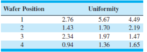
An article in the Journal of the Electrochemical Society (Vol. 139, No. 2, 1992, pp. 524–532) describes an experiment to investigate the low-pressure vapour deposition of polysilicon. The experiment was carried out in a large-capacity reactor at SEMATECH in Austin, Texas. The reactor has several wafer positions, and four of these positions are selected at random. The response variable is film thickness uniformity. Three replicates of the experiment were run, and the data are shown in Table 4E.8.
- (a) Is there a difference in the wafer positions? Use the analysis of variance and α = 0.05.
- (b) Estimate the variability due to wafer positions.
- (c) Estimate the random error component.
- (d) Analyze the residuals from this experiment and comment on model adequacy.
TABLE 4E.8
Uniformity Data for the Experiment in Exercise 4.42
Want to see the full answer?
Check out a sample textbook solution
Chapter 4 Solutions
Introduction to Statistical Quality Control
Additional Math Textbook Solutions
Introductory Statistics
Intro Stats, Books a la Carte Edition (5th Edition)
Elementary Statistics Using Excel (6th Edition)
Fundamentals of Statistics (5th Edition)
Basic Business Statistics, Student Value Edition


- In "Orthogonal Design for Process Optimization and Its Application to Plasma Etching" (Solid State Technology, May 1987), G. Z. Yin and D. W. Jillie describe an experiment to determine the effect of C2Fe flow rate on the uniformity of the etch on a silicon wafer used in integrated circuit manufacturing. Three flow rates are used in the experiment, and the resulting uniformity (in percent) for six replicates is shown below. Observations C„F. Flow (SCCM) 2 3 4 5 125 2.5 4.4 2.6 3.2 3.2 4.0 160 4.8 4.4 4.8 4.2 3.6 4.2 200 4.6 3.3 2.8 3.4 4.2 5.3 (a) Does C,F, flow rate affect etch uniformity? Construct box plots to compare the factor levels and perform the analysis of variance. Use a = 0.05. There is that flow rate affects etch uniformity. (b) Do the residuals indicate any problems with the underlying assumptions? No. Statistical Tables and Charts Yes.arrow_forwardIn Applied Spectroscopy, the infrared reflectance spectra properties of a viscous liquid used in the electronics industry as a lubricant were studied. The designed experiment consisted of the effect of band frequency x1 and film thickness x2 on optical density y using a Perkin-Elmer Model 621 infrared spectrometer. (Source: Pacansky, J., England, C. D., and Wattman, R., 1986.) y. Q4. 40 0.231 0.107 0.053 0.129 1.10 0.62 0.31 1.10 S05 S05 Sos 980 980 0.62 0.31 1.10 0.62 0.069 0.030 1.005 0.559 0.321 2.948 1.633 0.934 980 0.31 1.10 0.62 0.31 1235 1235 1235 Estimate the multiple linear regression equation.arrow_forwardPlease show me your solutions and interpretations. Show the completehypothesis-testing procedure.An article in the ASCE Journal of Energy Engineering (1999, Vol. 125, pp. 59–75) describes a study of the thermal inertia properties of autoclaved aerated concrete used as a building material. Five samples of the material were tested in a structure, and the average interior temperatures (°C) reported were as follows: 23.01, 22.22, 22.04, 22.62, and 22.59. Test that the average interior temperature is equal to 22.5 °C using α = 0.05.arrow_forward
- 2. Use the method of maximum likelihood to estimate 0 in the pdf V, y0. fr (y; 0) 2/y Evaluate 0e for the following random sample of size 4: yi 6, y2 = 8, y3 = 2.4, y4 = 5.9.arrow_forwardThe article "Measurements of the Thermal Conductivity and Thermal Diffusivity of Polymer Melts with the Short-Hot-Wire Method" (X. Zhang, W. Hendro, et al., International Journal of Thermophysics, 2002:1077-1090) reports measurements of the thermal conductivity (in W· m-1 . K') and diffusivity of several polymers at several temperatures (in 1000°C). The following table presents results for the thermal conductivity of polycarbonate. Cond. Temp. 0.236 0.028 0.241 0.038 0.244 0.061 0.251 0.083 0.259 0.107 0.257 0.119 0.257 0.130 0.261 0.146 0.254 0.159 0.256 0.169 0.251 0.181 0.249 0.204 0.249 0.215 0.230 0.225 0.230 0.237 0.228 0.248 Denoting conductivity by y and temperature by x, fit the linear model y = Bo + Bix + ɛ. a. For each coefficient, test the hypothesis that the coefficient is equal to 0. b. Fit the quadratic model y = Bo + Bix + Bzx? + ɛ. For each coefficient, test the Page 661 Fit the cubic model y = Bo + Bix + Bx + Bax + ɛ. For each coefficient, test the %3D hypothesis that…arrow_forwardThe management of the Seaside Golf Club regularly monitors the golfers on its course for speed of play. Suppose a random sample of golfers was taken in 2005 and another random sample of golfers was selected in 2006. The results of the two samples are as follows: 2005 2006 I2 = 219 S1 = 20.25 s2 = 21.70 n2 = 31 I = 225 %3D n1 = 36 Based on the sample results, can the management of the Seaside Golf Course conclude that the average speed of play was different in 2006 than in 2005? Conduct the appro- priate hypothesis test at the 0.10 level of significance. Assume that the management of the club is willing to accept the assumption that the populations of playing times for each year are approximately normally distributed.arrow_forward
- The article "Two Different Approaches for RDC Modelling When Simulating a Solvent Deasphalting Plant" (J. Aparicio, M. Heronimo, et al., Computers and Chemical Engineering, 2002:1369–1377) reports flow rate (in dmh) and specific gravity measurements for a sample of paraffinic hydrocarbons. The natural logs of the flow rates (y) and the specific gravity measurements (x) are presented in the following table. х -1.204 0.8139 -0.580 0.8171 0.049 0.8202 0 673 0.8233 1.311 0.8264 1.959 0.8294 2.614 0.8323 3.270 0.8352 Fit the linear model y = Bo + B,x + ɛ. For each coefficient, test the hypothesis that the coefficient is equal to 0. Fit the quadratic model y = Bo + B,x + B2x? + E. For each coefficient, test the a. b. hypothesis that the coefficient is equal to 0. Fit the cubic model y = Bo + Bix + B2x² + Bax + E. For each coefficient, test the C. hypothesis that the coefficient is equal to 0. Which of the models in parts (a) through (c) is the most appropriate? Explain. Using the most…arrow_forwardThe article in the ASCE Journal of Energy Engineering (1999, Vol. 125, pp.59-75) describes a study of the thermal inertia properties of autoclaved aerated concrete used as a building material. Five samples of the material were tested in a structure, and the average interior temperatures (°C) reported were as follows: 23.01, 22.22, 22.04, 22.62, and 22.59. Test that the average interior temperature is equal to 22.5°C using alpha (a) = 0.05. This problem is a test on what population parameter? What is the null and alternative hypothesis? What are the Significance level and type of test? What standardized test statistic will be used? What is the standard test statistic? What is the Statistical Decision? What is the statistical decision in the statement form?arrow_forwardAn article in Journal of Food Science [“Prevention of Potato Spoilage During Storage by Chlorine Dioxide” (2001, Vol. 66(3), pp. 472–477)] reported on a study of potato spoilage based on different conditions of acidified oxine (AO), which is a mixture of chlorite and chlorine dioxide. The data follow: ∑X1i=230, ∑X21i=17200, n1=3. ∑X2i=150, ∑X22i=8100, n2=3. ∑X3i=60, ∑X23i=4500, n3=3. ∑X4i=65, ∑X24i=1625, n4=3. where group 1 has AO = 50ppm, group 2 has AO = 100ppm, group 3 has AO = 200ppm, group 4 has AO = 400ppm. Complete the ANOVA table below Source df sum of square mean square F p-value Between Within N/A N/A Total 11 N/A N/A N/A At α=0.05, do we reject the null hypothesis that AO does not affect spoilage?arrow_forward
- A manufacturer is evaluating the variation in thickness for piezoelectric actuators from two component suppliers. The two populations are independent, and the thickness measurements are normally distributed. The thickness was measured for a sample of 30 products purchased from Supplier 1, and it was found that = 3.8048 . A sample of 30 products was also purchased from Supplier 2 and it was found that 5.2967. S1 S2 Is there evidence at the 0.1 level of significance that the thickness variance for Supplier 1 is smaller than for Supplier 2? (Round answers to 3 decimal places as needed) The correct alternative hypothesis is: O H1:0 + 0 OH1: H1 > µ2 : O H1:0} < o? O H1:0 2 0 O H1:0 O H1: µ1 2 l2 O H1: 41 < µ2 The test statistic is Fobs The probability of variance ratios at or beyond Fobs occurring by chance is = The decision is to Select an answer v that the variance in The correct summary would be: Select an answer thickness for Supplier 1 is smaller than Supplier 2.arrow_forwardThe article "Experimental Measurement of Radiative Heat Transfer in Gas-Solid Suspension Flow System" (G. Han, K. Tuzla, and J. Chen, AIChe Journal, 2002:1910- 1916) discusses the calibration of a radiometer. Several measurements were made on the electromotive force readings of the radiometer (in volts) and the radiation flux (in kilowatts per square meter). The results (read from a graph) are presented in the following table. Heat flux (y) 15 31 51 55 67 89 Signal output (x) 1.08 2.42 4.17 4.46 5.17 6.92 Compute the least-squares line for predicting heat flux from the signal output. If the radiometer reads 3.00 V, predict the heat flux. If the radiometer reads 8.00 V, should the heat flux be predicted? If so, predict it. If not, explain why. C.arrow_forward17.7 Butterfly wings. Researchers studied the morphological attributes of monarch butterflies (Danaus plexippus), a species that undertakes large seasonal migrations over North America. They measured the forewing weight (in milligrams, mg) of a sample of 92 monarch butterflies, all of which had been reared in captivity in identical conditions.° Figure 17.4 shows the output from the statistical software JMP. (The data are also available in the Large.Butterfly the data file if you wish to practice working with your own software.) Estimate with 95% confidence the mean forewing weight of monarch butterflies reared in captivity. Follow the four- step process as illustrated in Example 17.2. 4 STEP そMP FWweight 30 25 20 15 10 11 12 13 14 15 8 9 10 Summary Statistics Mean 11.795652 Std Dev 1.1759413 Std Err Mean 0.1226004 Upper 95% Mean Lower 95% Mean 1 FIGURE 17.4 Software output (JMP) for the forewing weight of monarch 12.039183 11.552122 92 N. butterflies. Countarrow_forward
 MATLAB: An Introduction with ApplicationsStatisticsISBN:9781119256830Author:Amos GilatPublisher:John Wiley & Sons Inc
 Probability and Statistics for Engineering and th...StatisticsISBN:9781305251809Author:Jay L. DevorePublisher:Cengage Learning
 Statistics for The Behavioral Sciences (MindTap C...StatisticsISBN:9781305504912Author:Frederick J Gravetter, Larry B. WallnauPublisher:Cengage Learning
 Elementary Statistics: Picturing the World (7th E...StatisticsISBN:9780134683416Author:Ron Larson, Betsy FarberPublisher:PEARSON
 The Basic Practice of StatisticsStatisticsISBN:9781319042578Author:David S. Moore, William I. Notz, Michael A. FlignerPublisher:W. H. Freeman
 Introduction to the Practice of StatisticsStatisticsISBN:9781319013387Author:David S. Moore, George P. McCabe, Bruce A. CraigPublisher:W. H. Freeman