
Videos
The article “Effect of Granular Subbase Thickness on Airfield Pavement Structural Response” (K. Gopalakrishnan and M. Thompson, Journal of Materials in Civil Engineering. 2008:331–342) presents a study of the effect of the subbase thickness (in mm) on the amount of surface deflection caused by aircraft landing on an airport runway. Two landing gears, one simulating a Boeing 747 aircraft, and the other a Boeing 777 aircraft, were trafficked across four test sections of runway. The results are presented in the following table.
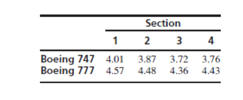
Can you conclude that the
Want to see the full answer?
Check out a sample textbook solution
Chapter 6 Solutions
Statistics for Engineers and Scientists
Additional Math Textbook Solutions
Elementary Statistics: Picturing the World (7th Edition)
PRACTICE OF STATISTICS F/AP EXAM
Business Statistics: A First Course (8th Edition)
Fundamentals of Statistics (5th Edition)


- The article "Experimental Measurement of Radiative Heat Transfer in Gas-Solid Suspension Flow System" (G. Han, K. Tuzla, and J. Chen, AIChe Journal, 2002:1910- 1916) discusses the calibration of a radiometer. Several measurements were made on the electromotive force readings of the radiometer (in volts) and the radiation flux (in kilowatts per square meter). The results (read from a graph) are presented in the following table. Heat flux (y) 15 31 51 55 67 89 Signal output (x) 1.08 2.42 4.17 4.46 5.17 6.92 Compute the least-squares line for predicting heat flux from the signal output. If the radiometer reads 3.00 V, predict the heat flux. If the radiometer reads 8.00 V, should the heat flux be predicted? If so, predict it. If not, explain why. C.arrow_forwardThe article “Effect of Granular Subbase Thickness on Airfield Pavement Structural Response” (K. Gopalakrishnan and M. Thompson, Journal of Materials in Civil Engineering, 2008:331–342) presents a study of the effect of the subbase thickness on the amount of surface deflection caused by aircraft landing on an airport runway. In six applications of a 160 kN load on a runway with a subbase thickness of 864 mm, the average surface deflection was 2.03 mm with a standard deviation of 0.090 mm. Find a 90% confidence interval for the mean deflection caused by a 160 kN load.arrow_forwardThe article "Modeling Resilient Modulus and Temperature Correction for Saudi Roads" (H. Wahhab, I. Asi, and R. Ramadhan, Journal of Materials in Civil Engineering, 2001:298– 305) describes a study designed to predict the resilient modulus of pavement from physical properties. The following table presents data for the resilient modulus at 40°Cin10® kPa (y), the surface area of the aggregate in m²/kg (x1), and the softening point of the asphalt in °C (х). y X1 X2 1.48 5.77 60.5 1.70 7.45 74.2 2.03 8.14 67.6 2.86 8.73 70.0 2.43 7.12 64.6 3.06 6.89 65.3 2.44 8.64 66.2 1.29 6.58 64.1 3.53 9.10 68.6 1.04 8.06 58.8 1.88 5.93 63.2 1.90 8.17 62.1 1.76 9.84 68.9 2.82 7.17 72.2 1.00 7.78 54.1 The full quadratic model is y = + P,x, + PzX, + Pz*jXz + Pxx¡ + Bzx; + €. Which submodel of this full model do you believe is most appropriate? Justify your answer by fitting two or more models and comparing the results.arrow_forward
- An article in the Fire Safety Journal (“The Effect of Nozzle Design on the Stability and Performance of Turbulent Water Jets,” Vol. 4, August 1981) describes an experiment in which a shape factor was determined for several different nozzle designs at six levels of jet efflux velocity. Interest focused on potential differences between nozzle designs (blocks), with velocity considered as a nuisance variable. The data are shown below: Jet Efflux Velocity (m/s) Nozzle Design 11.73 14.37 16.59 20.43 23.46 28.74 1 0.78 0.80 0.81 0.75 0.77 0.78 2 0.85 0.85 0.92 0.86 0.81 0.83 3 0.93 0.92 0.95 0.89 0.89 0.83 4 1.14 0.97 0.98 0.88 0.86 0.83 5 0.97 0.86 0.78 0.76 0.76 0.75 1) Write the null hypothesis and the alternative hypothesis (for the factor). 2) Find the ANOVA table. (round to five decimal places). 3) What is your decision about the null hypothesis, consider ?. 4) If your decision in part (4) was reject , perform Tukey test to determine which pairwise means are…arrow_forwardThe article "Influence of Freezing Temperature on Hydraulic Conductivity of Silty Clay" (J. Konrad and M. Samson, Journal of Geotechnical and Geoenvironmental Engineering, 2000:180–187) describes a study of factors affecting hydraulic conductivity of soils. The measurements of hydraulic conductivity in units of 108 cm/s (y), initial void ratio (x), and thawed void ratio (x2) for 12 specimens of silty clay are presented in the following table. y 1.01 1.12 1.04 1.30 1.01 1.04 0.955 1.15 1.23 1.28 1.23 1.30 0.84 0.88 0.85 0.95 0.88 0.86 0.85 0.89 0.90 0.94 0.88 0.90 X1 0.81 0.85 0.87 0.92 0.84 0.85 0.85 0.86 0.85 0.92 0.88 0.92 X2 Fit the model y = Bo + fix1 + e. For each coefficient, test the null hypothesis that it is equal to 0. Fit the model y = Bo + Bzx2 + e. For each coefficient, test the null hypothesis that it is equal to 0. Fit the model y = Bo + BzX1 + Bzxz + e. For each coefficient, test the null hypothesis that it is equal to 0. d. Which of the models in parts (a) to (c) is…arrow_forwardThe article "Modeling of Urban Area Stop-and-Go Traffic Noise" (P. Pamanikabud and C. Tharasawatipipat, Journal of Transportation Engineering, 1999:152–159) presents measurements of traffic noise, in dBA, from 10 locations in Bangkok, Thailand. Measurements, presented in the following table, were made at each location, in both the acceleration and deceleration lanes. Location Acceleration Deceleration 78.1 78.6 78.1 80.0 3 79.6 79.3 4 81.0 79.1 78.7 78.2 78.1 78.0 78.6 78.6 78.5 78.8 78.4 78.0 10 79.6 78.4 Can you conclude that there is a difference in the mean noise levels between acceleration and deceleration lanes?arrow_forward
- Please show me your solutions and interpretations. Show the completehypothesis-testing procedure.An article in the ASCE Journal of Energy Engineering (1999, Vol. 125, pp. 59–75) describes a study of the thermal inertia properties of autoclaved aerated concrete used as a building material. Five samples of the material were tested in a structure, and the average interior temperatures (°C) reported were as follows: 23.01, 22.22, 22.04, 22.62, and 22.59. Test that the average interior temperature is equal to 22.5 °C using α = 0.05.arrow_forwardThe article "Effect of Microstructure and Weathering on the Strength Anisotropy of Porous Rhyolite" (Y. Matsukura, K. Hashizume, and C. Oguchi, Engineering Geology, 2002:39- 17) investigates the relationship between the angle betwween cleavage and flow structure and the strength of porous rhyolite. Strengths (in MPa) were measured for a mumber of specimens cut at various angles. The mean and standard deviation of the strengths for each angle are presented in the following table. Angle Mean 0° 22.9 Sample Size Standard Deviation 2.98 12 15° 22.9 1.16 30° 19.7 3.00 45° 14.9 2.99 60° 13.5 2.33 75° 11.9 2.10 90 14.3 3.95 6. Can you conclude that strength varies with the angle?arrow_forwardArtificial joints consist of a ceramic ball mounted on a taper. The article "Friction in Orthopaedic Zirconia Taper Assemblies" (W. Macdonald, A. Áspenberg, et al., Proceedings of the Institution of Mechanical Engineers, 2000: 685-692) presents data on the coefficient of friction for a push-on load of 2 kN for taper assemblies made from two zirconium alloys and employing three different neck lengths. Five measurements were made for each combination of material and neck length. The results presented in the following table are consistent with the cell means and standard deviations presented in the article. Тарег Material Neck Length Coefficient of Friction CPTI-ZIO2 CPTI-Z:O, CPTI-Z:O, Long TIAlloy-ZrO, Short TiAlloy-ZrO, Medium TiAlloy-ZrO, Long Short 0.254 0.195 0.281 0.289 0.220 Medium 0.196 0.220 0.185 0.259 0.197 0.329 0.481 0.320 0.296 0.178 0.150 0.118 0.158 0.175 0.131 0.180 0.184 0.154 0.156 0.177 0.178 0.198 0.201 0.199 0.210 Compute the main effects and interactions. Construct…arrow_forward
- Wrinkle recovery angle and tensile strength are the two most important characteristics for evaluating the performance of crosslinked cotton fabric. An increase in the degree of crosslinking, as determined by ester carboxyl band absorbance, improves the wrinkle resistance of the fabric (at the expense of reducing mechanical strength). The accompanying data on x = absorbance and y = wrinkle resistance angle was read from a graph in the paper "Predicting the Performance of Durable Press Finished Cotton Fabric with Infrared Spectroscopy".† x 0.115 0.126 0.183 0.246 0.282 0.344 0.355 0.452 0.491 0.554 0.651 y 334 342 355 363 365 372 381 392 400 412 420 Here is regression output from Minitab: Predictor Constant absorb S = 3.60498 Coef 321.878 156.711 SOURCE Regression Residual Error Total SE Coef 2.483 6.464 R-Sq = 98.5% DF 1 9 10 SS 7639.0 117.0 7756.0 T 129.64 24.24 0.000 0.000 R-Sq (adj) = 98.3% MS 7639.0 13.0 F P 587.81 (a) Does the simple linear regression model appear to be…arrow_forwardWrinkle recovery angle and tensile strength are the two most important characteristics for evaluating the performance of crosslinked cotton fabric. An increase in the degree of crosslinking, as determined by ester carboxyl band absorbance, improves the wrinkle resistance of the fabric (at the expense of reducing mechanical strength). The accompanying data on x = absorbance and y = wrinkle resistance angle was read from a graph in the paper "Predicting the Performance of Durable Press Finished Cotton Fabric with Infrared Spectroscopy".t x 0.115 0.126 0.183 0.246 0.282 0.344 0.355 0.452 0.491 0.554 0.651 y 334 342 355 363 365 372 381 400 392 412 420 Here is regression output from Minitab: Predictor Constant absorb S = 3.60498 Coef 321.878 156.711 SOURCE Regression Residual Error Total R-Sq= 98.5% DF SE Coef 2.483 6.464 1 9 10 SS 7639.0 117.0 7756..0 T 129.64 24.24 P 0.000 0.000. R-Sq (adj) 98.3% MS 7639.0 13.0 F 587.81 (a) Does the simple linear regression model appear to be appropriate?…arrow_forwardThe article "Drying of Pulps in Sprouted Bed: Effect of Composition on Dryer Performance" (M. Medeiros, S. Rocha, et al., Drying Technology, 2002:865-881) presents measurements of pH, viscosity (in kg/m - s), density (in g/cm), and BRIX (in percent). The following MINITAB output presents the results of fitting the model pH = 6, +6, Viscosity + B, Density + ß, BRIX +€ The regression equation is pH - -1.79 + 0.000266 Viscosity + 9.82 Density - 0.300 BRIX Predictor Coef SE Coef Constant -1.7914 6.2339 -0.29 0.778 Viscosity 0.00026626 0.00011517 2.31 0.034 Density 9.8184 5.7173 1.72 0.105 BRIX -0.29982 0.099039 -3.03 0.008 S - 0.379578 R-Sq - 50.0% R-Sq(adj) - 40.6% Predicted Values for New Observations New Obs Fit SE Fit 95% CI 95% PI 3.0875 0.1351 (2.8010, 3.3740) (2.2333, 3.9416) (3.4207, 4.0496) (2.3255, 3.3896) 2 3.7351 0.1483 (2.8712, 4.5990) з 2.8576 0.2510 (1.8929, 3.8222) Values of Predictors for New Observations New Obs Viscosity Density BRIX 1000 1.05 19.0 1200 1.08 18.0 2000…arrow_forward
 MATLAB: An Introduction with ApplicationsStatisticsISBN:9781119256830Author:Amos GilatPublisher:John Wiley & Sons Inc
 Probability and Statistics for Engineering and th...StatisticsISBN:9781305251809Author:Jay L. DevorePublisher:Cengage Learning
 Statistics for The Behavioral Sciences (MindTap C...StatisticsISBN:9781305504912Author:Frederick J Gravetter, Larry B. WallnauPublisher:Cengage Learning
 Elementary Statistics: Picturing the World (7th E...StatisticsISBN:9780134683416Author:Ron Larson, Betsy FarberPublisher:PEARSON
 The Basic Practice of StatisticsStatisticsISBN:9781319042578Author:David S. Moore, William I. Notz, Michael A. FlignerPublisher:W. H. Freeman
 Introduction to the Practice of StatisticsStatisticsISBN:9781319013387Author:David S. Moore, George P. McCabe, Bruce A. CraigPublisher:W. H. Freeman