
Videos
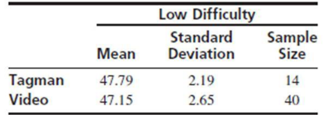
The article “Time Series Analysis for Construction Productivity Experiments” (T. Abdelhamid and J. Everett. Journal of Construction Engineering and Management. 1999:87–95) presents a study comparing the effectiveness of a video system that allows a crane operator to see the lifting point while operating the crane with the old system in which the operator relies on hand signals from a tagman. Three different lifts, A, B, and C, were studied. Lift A was of little difficulty, lift B was of moderate difficulty, and lift C was of high difficulty. Each lift was performed several times, both with the new video system and with the old tagman system. The time (in seconds) required to perform each lift was recorded. The following tables present the means, standard deviations, and
- a. Can you conclude that the
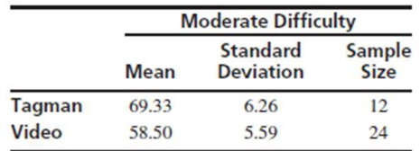
mean time to perform a lift of low difficulty is less when using the video system than when using the tagman system? Explain. - b. Can you conclude that the mean time to perform a lift of moderate difficulty is less when using the video system than when using the tagman system? Explain.
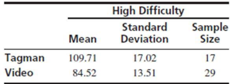
- c. Can you conclude that the mean time to perform a lift of high difficulty is less when using the video system than when using the tagman system? Explain.
a.
Check whether there is evidence to conclude that the mean time to perform a lift of low difficulty is less when using the video system than when using the tagman system.
Answer to Problem 4E
There is no evidence to conclude that the mean time to perform a lift of low difficulty is less when using the video system than when using the tagman system.
Explanation of Solution
Given info:
Three different lifts, A, B, and C, were studied in the given experiment. Lift A was of little difficulty, lift B was of moderate difficulty, and lift C was of high difficulty. The summary statistics for three lifts are given below:
Low difficulty:
Tagman:
Video:
Moderate difficulty:
Tagman:
Video:
High difficulty:
Tagman:
Video:
Calculation:
State the test hypotheses.
Null hypothesis:
Alternative hypothesis:
Tests statistic and P-value:
Software Procedure:
Step-by-step procedure to obtain the test statistic using the MINITAB software:
- Choose Stat > Basic Statistics > 2-Sample t.
- Choose Summarized data.
- In first, enter Sample size as 14, Mean as 47.79, Standard deviation as 2.19.
- In second, enter Sample size as 40, Mean as 47.15, Standard deviation as 2.65.
- Choose Options.
- In Confidence level, enter 95.
- In Alternative, select greater than.
- Click OK in all the dialogue boxes.
Output using the MINITAB software is given below:
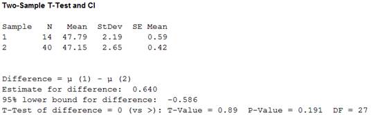
From the MINITAB output, the test statistic is 0.89 and the P-value is 0.191.
Conclusion:
The P-value is 0.191 and the significance level is 0.05.
Here, the P-value is greater than the significance level.
That is,
Therefore, the null hypothesis is not rejected.
Thus, there is no evidence to conclude that the mean time to perform a lift of low difficulty is less when using the video system than when using the tagman system.
b.
Check whether there is evidence to conclude that the mean time to perform a lift of moderate difficulty is less when using the video system than when using the tagman system.
Answer to Problem 4E
There is evidence to conclude that the mean time to perform a lift of moderate difficulty is less when using the video system than when using the tagman system.
Explanation of Solution
Calculation:
State the test hypotheses.
Null hypothesis:
Alternative hypothesis:
Tests statistic and P-value:
Software Procedure:
Step-by-step procedure to obtain the test statistic using the MINITAB software:
- Choose Stat > Basic Statistics > 2-Sample t.
- Choose Summarized data.
- In first, enter Sample size as 12, Mean as 69.33, Standard deviation as 6.26.
- In second, enter Sample size as 24, Mean as 58.50, Standard deviation as 5.59.
- Choose Options.
- In Confidence level, enter 95.
- In Alternative, select greater than.
- Click OK in all the dialogue boxes.
Output using the MINITAB software is given below:
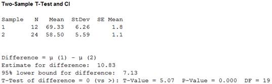
From the MINITAB output, the test statistic is 5.07 and the P-value is 0.000.
Conclusion:
The P-value is 0.000 and the significance level is 0.05.
Here, the P-value is less than the significance level.
That is,
Therefore, the null hypothesis is rejected.
Thus, there is evidence to conclude that the mean time to perform a lift of moderate difficulty is less when using the video system than when using the tagman system.
c.
Check whether there is evidence to conclude that the mean time to perform a lift of high difficulty is less when using the video system than when using the tagman system.
Answer to Problem 4E
There is evidence to conclude that the mean time to perform a lift of high difficulty is less when using the video system than when using the tagman system.
Explanation of Solution
Calculation:
State the test hypotheses.
Null hypothesis:
Alternative hypothesis:
Tests statistic and P-value:
Software Procedure:
Step-by-step procedure to obtain the test statistic using the MINITAB software:
- Choose Stat > Basic Statistics > 2-Sample t.
- Choose Summarized data.
- In first, enter Sample size as 17, Mean as 109.71, Standard deviation as 17.02.
- In second, enter Sample size as 29, Mean as 84.52, Standard deviation as 13.51.
- Choose Options.
- In Confidence level, enter 95.
- In Alternative, select greater than.
- Click OK in all the dialogue boxes.
Output using the MINITAB software is given below:
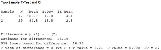
From the MINITAB output, the test statistic is 5.21 and the P-value is 0.000.
Conclusion:
The P-value is 0.000 and the significance level is 0.05.
Here, the P-value is less than the significance level.
That is,
Therefore, the null hypothesis is rejected.
Thus, there is evidence to conclude that the mean time to perform a lift of high difficulty is less when using the video system than when using the tagman system.
Want to see more full solutions like this?
Chapter 6 Solutions
Statistics for Engineers and Scientists
Additional Math Textbook Solutions
Essential Statistics
Business Analytics
Elementary Statistics Using The Ti-83/84 Plus Calculator, Books A La Carte Edition (5th Edition)
Developmental Mathematics (9th Edition)
Essentials of Statistics (6th Edition)
Business Statistics: A First Course (8th Edition)


- A paper investigated the driving behavior of teenagers by observing their vehicles as they left a high school parking lot and then again at a site approximately 1 2 mile from the school. Assume that it is reasonable to regard the teen drivers in this study as representative of the population of teen drivers. MaleDriver FemaleDriver 1.3 -0.3 1.3 0.6 0.9 1.1 2.1 0.7 0.7 1.1 1.3 1.2 3 0.1 1.3 0.9 0.6 0.5 2.1 0.5 (a) Use a .01 level of significance for any hypothesis tests. Data consistent with summary quantities appearing in the paper are given in the table. The measurements represent the difference between the observed vehicle speed and the posted speed limit (in miles per hour) for a sample of male teenage drivers and a sample of female teenage drivers. (Use ?males − ?females. Round your test statistic to two decimal places. Round your degrees of freedom down to the nearest whole number. Round your p-value to three decimal places.) t = df =…arrow_forward27. An article in Radio Engineering and Electronic Physics (1980, Vol. 25, pp. 74-79) investigated the behavior of a stochastic generator in the presence of external noise. The number of periods was measured in a sample of 100 trains for each of two different levels of noise voltage, 100 and 150 mV. For 100 mV, the mean number of periods in a train was 7.9 with s1 = 2.6. For 150 mV, the mean was 6.9 with s2 = 2.4. Use α = 0.01 and assume that each population is normally distributed and the two population variances are equal. (a) It was originally suspected that raising noise voltage would reduce mean number of periods. Do the data support this claim? (b) Calculate a confidence interval to answer the question in part (a).arrow_forwardThe article “Effects of Diets with Whole Plant-Origin Proteins Added with Different Ratiosof Taurine:Methionine on the Growth, Macrophage Activity and Antioxidant Capacity ofRainbow Trout (Oncorhynchus mykiss) Fingerlings” (O. Hernandez, L. Hernandez, et al.,Veterinary and Animal Science, 2017:4-9) reports that a sample of 210 juvenile rainbowtrout fed a diet fortified with equal amounts of the amino acids taurine and methionine for aperiod of 70 days had a mean weight gain of 313 percent with a standard deviation of 25, while 210 fish fed with a control diet had a mean weight gain of 233 percent with a standard deviation of 19. Units are percent. Find a 99% confidence interval for the difference in weight gain on the two diets.arrow_forward
- A local church is interested in determining how length of residence in the present community relates to church attendance. Using a random sample of 15 individuals, they gathered data on how many times in the previous 5 weeks each individual attended church services. The data are provided below. Length of residence in the community Less than 2 years 2-5 years More than 5 years 0 0 1 1 2 3 3 3 3 4 4 4 4 5 4 Using the 5-step model, determine whether and how church attendance is related to length of residence in the community. Use 5% and 1% levels of statistical significance. What are the assumptions for this problem?arrow_forwardQuestion 2 A researcher was interested in studying if there is a significant relationship between the severity of COVID 19 and blood types of individuals. 2400 individuals were studied and the results are shown below. Condition Blood Type O A B AB Total Critical 64 44 20 8 136 Severe 175 129 50 15 369 Moderate 211 528 151 125 1015 Mild 200 400 140 140 880 Total 650 1101 361 288 240 a .State both the null and alternative hypotheses. b. Provide the decision rule for making this decision. Use an alpha level of 5%. c. Show all of the work necessary to calculate the appropriate statistic.d. What conclusion are you allowed to draw? e. Would your conclusion change at the 10% level of significance?arrow_forwardThe males of stalk-eyed flies (Cyrtodiopsis dalmanni) have long eye stalks. The females sometimes use the length of these eye stalks to choose mates. Is the male’s eye-stalk length affected by the quality of its diet? An experiment was carried out in which two groups of male “stalkies” were reared on different foods (David et al. 2000). One group was fed “corn” (considered a high quality food), while the other was fed “cotton” wool (a food of substantially lower quality). Each male was raised singly and so represents an independent sampling unit. The eye spans (the distance between the eyes) were recorded in millimeters. The raw data, which are plotted as histograms below, are as follows: Corn diet: 2.15, 2.14, 2.13, 2.13, 2.12, 2.11, 2.1, 2.08, 2.08, 2.08, 2.04, 2.05, 2.03, 2.02, 2.01, 2, 1.99, 1.96, 1.95, 1.93, 1.89Cotton diet: 2.12, 2.07, 2.01, 1.93, 1.77, 1.68, 1.64, 1.61, 1.59, 1.58, 1.56, 1.55, 1.54, 1.49, 1.45, 1.43, 1.39, 1.34, 1.33, 1.29, 1.26, 1.24, 1.11, 1.05 a) what is the…arrow_forward
- A sample of 26 offshore oil workers took part in a simulated escape exercise, resulting in the accompanying data on time (sec) to complete the escape (“Oxygen Consumption and Ventilation During Escape from an Offshore Platform,” Ergonomics, 1997: 281-292): 389 356 359 363 375 424 325 394 402 373 373 370 364 366 364 325 339 393 392 369 374 359 356 403 334 397 a. Construct a stem-and-leaf display of the data. How does it suggest that the sample mean and median will compare?b. Calculate the values of the sample mean and median. [Hint: Σxi = 9638.]c. By how much could the largest time, currently 424, be increased without affecting the value of the sample median? By how much could this value be decreased without affecting the value of the sample median?d. What are the values of x and x when the observations are reexpressed in minutes?arrow_forwardA U.S. Food Survey showed that Americans routinely eat beef in their diet. Suppose that in a study of 49 consumers in Illinois and 64 consumers in Texas the following results were obtained from two samples regarding average yearly beef consumption: Illinois Texas = 49 = 64 = 54.1lb = 60.4lb S1 = 7.0 S2 = 8.0 Formulate a hypothesis so that, if the null hypothesis is rejected, we can conclude that the average amount of beef eaten annually by consumers in Illinois is significantly less than that eaten by consumers in Texas.arrow_forwardIn the book Business Research Methods (5th ed.), Donald R. Cooper and C. William Emory discuss studying the relationship between on-the-job accidents and smoking. Cooper and Emory describe the study as follows: Suppose a manager implementing a smoke-free workplace policy is interested in whether smoking affects worker accidents. Since the company has complete reports of on-the-job accidents, she draws a sample of names of workers who were involved in accidents during the last year. A similar sample from among workers who had no reported accidents in the last year is drawn. She interviews members of both groups to determine if they are smokers or not. The sample results are given in the following table. On-the-Job Accident Smoker Yes No Row Total Heavy 12 5 17 Moderate 9 10 19 Nonsmoker 13 17 30 Column total 34 32 66 Expected counts are below observed counts Accident No Accident Total Heavy 12 5 17 8.76 8.24…arrow_forward
- A paper investigated the driving behavior of teenagers by observing their vehicles as they left a high school parking lot and then again at a site approximately 1 2 mile from the school. Assume that it is reasonable to regard the teen drivers in this study as representative of the population of teen drivers. Amount by Which Speed Limit Was Exceeded MaleDriver FemaleDriver 1.2 -0.1 1.4 0.4 0.9 1.1 2.1 0.7 0.7 1.1 1.3 1.2 3 0.1 1.3 0.9 0.6 0.5 2.1 0.5 (a) Use a .01 level of significance for any hypothesis tests. Data consistent with summary quantities appearing in the paper are given in the table. The measurements represent the difference between the observed vehicle speed and the posted speed limit (in miles per hour) for a sample of male teenage drivers and a sample of female teenage drivers. (Use μmales − μfemales.Round your test statistic to two decimal places. Round your degrees of freedom down to the nearest whole number. Round your p-value to…arrow_forwardA paper investigated the driving behavior of teenagers by observing their vehicles as they left a high school parking lot and then again at a site approximately 1 2 mile from the school. Assume that it is reasonable to regard the teen drivers in this study as representative of the population of teen drivers. Amount by Which Speed Limit Was Exceeded MaleDriver FemaleDriver 1.3 -0.1 1.3 0.4 0.9 1.1 2.1 0.7 0.7 1.1 1.3 1.2 3 0.1 1.3 0.9 0.6 0.5 2.1 0.5 (a) Use a .01 level of significance for any hypothesis tests. Data consistent with summary quantities appearing in the paper are given in the table. The measurements represent the difference between the observed vehicle speed and the posted speed limit (in miles per hour) for a sample of male teenage drivers and a sample of female teenage drivers. (Use μmales − μfemales.Round your test statistic to two decimal places. Round your degrees of freedom down to the nearest whole number. Round your p-value to…arrow_forwardThe following data represents results from an experiment comparing 3 treatment conditions for the cure of boredom. Treatment 1 is doing schoolwork, Treatment 2 is watching tv, and Treatment 3 is spending time with friends. The following scores represent treatment effectiveness scores where higher values indicate that the treatment of boredom was effective and lower values indicate that the treatment of boredom was ineffective. Treatment 1 Treatment 2 Treatment 3 0 1 6 N= 12 1 4 5 GM= 3.00 0 1 8 3 2 5…arrow_forward
 MATLAB: An Introduction with ApplicationsStatisticsISBN:9781119256830Author:Amos GilatPublisher:John Wiley & Sons Inc
 Probability and Statistics for Engineering and th...StatisticsISBN:9781305251809Author:Jay L. DevorePublisher:Cengage Learning
 Statistics for The Behavioral Sciences (MindTap C...StatisticsISBN:9781305504912Author:Frederick J Gravetter, Larry B. WallnauPublisher:Cengage Learning
 Elementary Statistics: Picturing the World (7th E...StatisticsISBN:9780134683416Author:Ron Larson, Betsy FarberPublisher:PEARSON
 The Basic Practice of StatisticsStatisticsISBN:9781319042578Author:David S. Moore, William I. Notz, Michael A. FlignerPublisher:W. H. Freeman
 Introduction to the Practice of StatisticsStatisticsISBN:9781319013387Author:David S. Moore, George P. McCabe, Bruce A. CraigPublisher:W. H. Freeman