Concept explainers
Videos
(a)
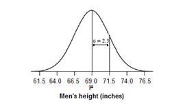
To find: the percent of men who are taller than 74 inches
(a)
Answer to Problem 43E
Approximately 2.5 % of men are taller than 74 inches.
Explanation of Solution
Calculation:
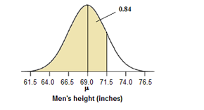
The distribution of heights is approximately N (69, 2.5). Figure below is a sketch of the Normaldensity curve with the desired points labeled.
By the
Conclusion:
Therefore,2.5% of men are taller than 74 inches
(b)
To find: the height
(b)
Answer to Problem 43E
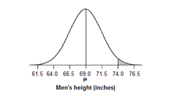
Approximately 95% of men have heights between 64 inches and 74 inches.
Explanation of Solution
Calculation:
By the 68-95-99.7 rule, approximately 95% of men have heights between 64 inches and 74inches which fall within 2s of µ.
Conclusion:
Therefore, 95% of men have heights between 64 inches and 74inches
(c)
To find: the percent of men who arebetween 64 and 66.5 inches tall
(c)
Answer to Problem 43E
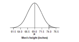
Approximately16% -2.5% = 13.5% of men have heights between 64 inches and 66.5 inches.
Explanation of Solution
Calculation:
By the 68-95-99.7 rule, approximately 16% of men are shorter than 66.5 inches, because66.5 is one standard deviation below the mean. Approximately 2.5% are shorter than 64 inches,because 64 inches is two standard deviations below the mean. So approximately 16% - 2.5% = 13.5% of men have heights between 64 inches and 66.5 inches.
Conclusion:
Therefore, 16% -2.5% = 13.5% of men have heights between 64 inches and 66.5 inches.
(d)
To find: the percentile of adult male American heights corresponding to 71.5 inches height.
(d)
Answer to Problem 43E
Here, 71.5 is the 84th percentile of adult male American heights.
Explanation of Solution
Calculation:
By the 68-95-99 .7 rule, the value 71.5 is one standard deviation above the mean. Thus, the area to the left of 71.5is 0.68 +0.16 = 0.84. In other words, 71.5 is the 84th percentile of adult male American heights.
Conclusion:
Therefore, 71.5 is the 84th percentile of adult male American heights.
Chapter 2 Solutions
The Practice of Statistics for AP - 4th Edition
Additional Math Textbook Solutions
Algebra and Trigonometry (6th Edition)
College Algebra with Modeling & Visualization (5th Edition)
Calculus for Business, Economics, Life Sciences, and Social Sciences (14th Edition)
Introductory Statistics
Elementary Statistics (13th Edition)


- What is one sample T-test? Give an example of business application of this test? What is Two-Sample T-Test. Give an example of business application of this test? .What is paired T-test. Give an example of business application of this test? What is one way ANOVA test. Give an example of business application of this test? 1. One Sample T-Test: Determine whether the average satisfaction rating of customers for a product is significantly different from a hypothetical mean of 75. (Hints: The null can be about maintaining status-quo or no difference; If your alternative hypothesis is non-directional (e.g., μ≠75), you should use the two-tailed p-value from excel file to make a decision about rejecting or not rejecting null. If alternative is directional (e.g., μ < 75), you should use the lower-tailed p-value. For alternative hypothesis μ > 75, you should use the upper-tailed p-value.) H0 = H1= Conclusion: The p value from one sample t-test is _______. Since the two-tailed p-value…arrow_forwardUsing the accompanying Accounting Professionals data to answer the following questions. a. Find and interpret a 90% confidence interval for the mean years of service. b. Find and interpret a 90% confidence interval for the proportion of employees who have a graduate degree. view the Accounting Professionals data. Employee Years of Service Graduate Degree?1 26 Y2 8 N3 10 N4 6 N5 23 N6 5 N7 8 Y8 5 N9 26 N10 14 Y11 10 N12 8 Y13 7 Y14 27 N15 16 Y16 17 N17 21 N18 9 Y19 9 N20 9 N Question content area bottom Part 1 a. A 90% confidence interval for the mean years of service is (Use ascending order. Round to two decimal places as needed.)arrow_forwardIf, based on a sample size of 900,a political candidate finds that 509people would vote for him in a two-person race, what is the 95%confidence interval for his expected proportion of the vote? Would he be confident of winning based on this poll? Question content area bottom Part 1 A 9595% confidence interval for his expected proportion of the vote is (Use ascending order. Round to four decimal places as needed.)arrow_forward
- Questions An insurance company's cumulative incurred claims for the last 5 accident years are given in the following table: Development Year Accident Year 0 2018 1 2 3 4 245 267 274 289 292 2019 255 276 288 294 2020 265 283 292 2021 263 278 2022 271 It can be assumed that claims are fully run off after 4 years. The premiums received for each year are: Accident Year Premium 2018 306 2019 312 2020 318 2021 326 2022 330 You do not need to make any allowance for inflation. 1. (a) Calculate the reserve at the end of 2022 using the basic chain ladder method. (b) Calculate the reserve at the end of 2022 using the Bornhuetter-Ferguson method. 2. Comment on the differences in the reserves produced by the methods in Part 1.arrow_forwardA population that is uniformly distributed between a=0and b=10 is given in sample sizes 50( ), 100( ), 250( ), and 500( ). Find the sample mean and the sample standard deviations for the given data. Compare your results to the average of means for a sample of size 10, and use the empirical rules to analyze the sampling error. For each sample, also find the standard error of the mean using formula given below. Standard Error of the Mean =sigma/Root Complete the following table with the results from the sampling experiment. (Round to four decimal places as needed.) Sample Size Average of 8 Sample Means Standard Deviation of 8 Sample Means Standard Error 50 100 250 500arrow_forwardA survey of 250250 young professionals found that two dash thirdstwo-thirds of them use their cell phones primarily for e-mail. Can you conclude statistically that the population proportion who use cell phones primarily for e-mail is less than 0.720.72? Use a 95% confidence interval. Question content area bottom Part 1 The 95% confidence interval is left bracket nothing comma nothing right bracket0.60820.6082, 0.72510.7251. As 0.720.72 is within the limits of the confidence interval, we cannot conclude that the population proportion is less than 0.720.72. (Use ascending order. Round to four decimal places as needed.)arrow_forward
- I need help with this problem and an explanation of the solution for the image described below. (Statistics: Engineering Probabilities)arrow_forwardA survey of 250 young professionals found that two-thirds of them use their cell phones primarily for e-mail. Can you conclude statistically that the population proportion who use cell phones primarily for e-mail is less than 0.72? Use a 95% confidence interval. Question content area bottom Part 1 The 95% confidence interval is [ ], [ ] As 0.72 is ▼ above the upper limit within the limits below the lower limit of the confidence interval, we ▼ can cannot conclude that the population proportion is less than 0.72. (Use ascending order. Round to four decimal places as needed.)arrow_forwardI need help with this problem and an explanation of the solution for the image described below. (Statistics: Engineering Probabilities)arrow_forward
- I need help with this problem and an explanation of the solution for the image described below. (Statistics: Engineering Probabilities)arrow_forwardI need help with this problem and an explanation of the solution for the image described below. (Statistics: Engineering Probabilities)arrow_forwardQuestions An insurance company's cumulative incurred claims for the last 5 accident years are given in the following table: Development Year Accident Year 0 2018 1 2 3 4 245 267 274 289 292 2019 255 276 288 294 2020 265 283 292 2021 263 278 2022 271 It can be assumed that claims are fully run off after 4 years. The premiums received for each year are: Accident Year Premium 2018 306 2019 312 2020 318 2021 326 2022 330 You do not need to make any allowance for inflation. 1. (a) Calculate the reserve at the end of 2022 using the basic chain ladder method. (b) Calculate the reserve at the end of 2022 using the Bornhuetter-Ferguson method. 2. Comment on the differences in the reserves produced by the methods in Part 1.arrow_forward
 MATLAB: An Introduction with ApplicationsStatisticsISBN:9781119256830Author:Amos GilatPublisher:John Wiley & Sons Inc
 Probability and Statistics for Engineering and th...StatisticsISBN:9781305251809Author:Jay L. DevorePublisher:Cengage Learning
 Statistics for The Behavioral Sciences (MindTap C...StatisticsISBN:9781305504912Author:Frederick J Gravetter, Larry B. WallnauPublisher:Cengage Learning
 Elementary Statistics: Picturing the World (7th E...StatisticsISBN:9780134683416Author:Ron Larson, Betsy FarberPublisher:PEARSON
 The Basic Practice of StatisticsStatisticsISBN:9781319042578Author:David S. Moore, William I. Notz, Michael A. FlignerPublisher:W. H. Freeman
 Introduction to the Practice of StatisticsStatisticsISBN:9781319013387Author:David S. Moore, George P. McCabe, Bruce A. CraigPublisher:W. H. Freeman