Chapter 2.2, Problem 2.1CYU

To determine

Proportion of observations that fall under the standard normal region z <1.39

Answer to Problem 2.1CYU

Proportion of observations from a standard normal distribution that fall under the region z <1.39 is91.77%.

Explanation of Solution

The area under standard normal curve is drawn using Desmos software and shaded. The area under normal curve is the shaded region to the left of 1.39 in the graph.

The corresponding probability is read using table A. The observation corresponding row heading 1.30 (under column z) and column heading .09 is the area under normal curve. It is also proportion of observations which fall under the region z <1.39. The value is 0.9177. Hence proportion of observations from a standard normal distribution that fall under the region z <1.39 is 0.9177 or 91.77%.

  

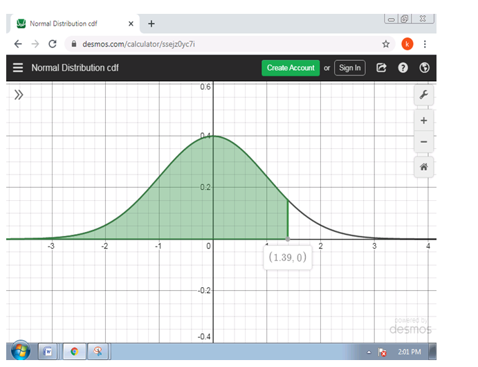
Conclusion: Proportion of observations that fall under the standard normal region z <1.39 is 91.77%