
Introduction To Statistics And Data Analysis
6th Edition
ISBN: 9781337793612
Author: PECK, Roxy.
Publisher: Cengage Learning,
expand_more
expand_more
format_list_bulleted
Concept explainers
Videos
Textbook Question
Chapter 14, Problem 73CR
This exercise requires the use of a statistical software package. The article “Entry and Profitability in a Rate-Free Savings and Loan Market” (Quarterly Review of Economics and Business [1978]: 87–95) gave the accompanying data on y = Profit margin of savings and loan companies in a given year, x1 = Net revenues in that year, and x2 = Number of savings and loan branch offices.
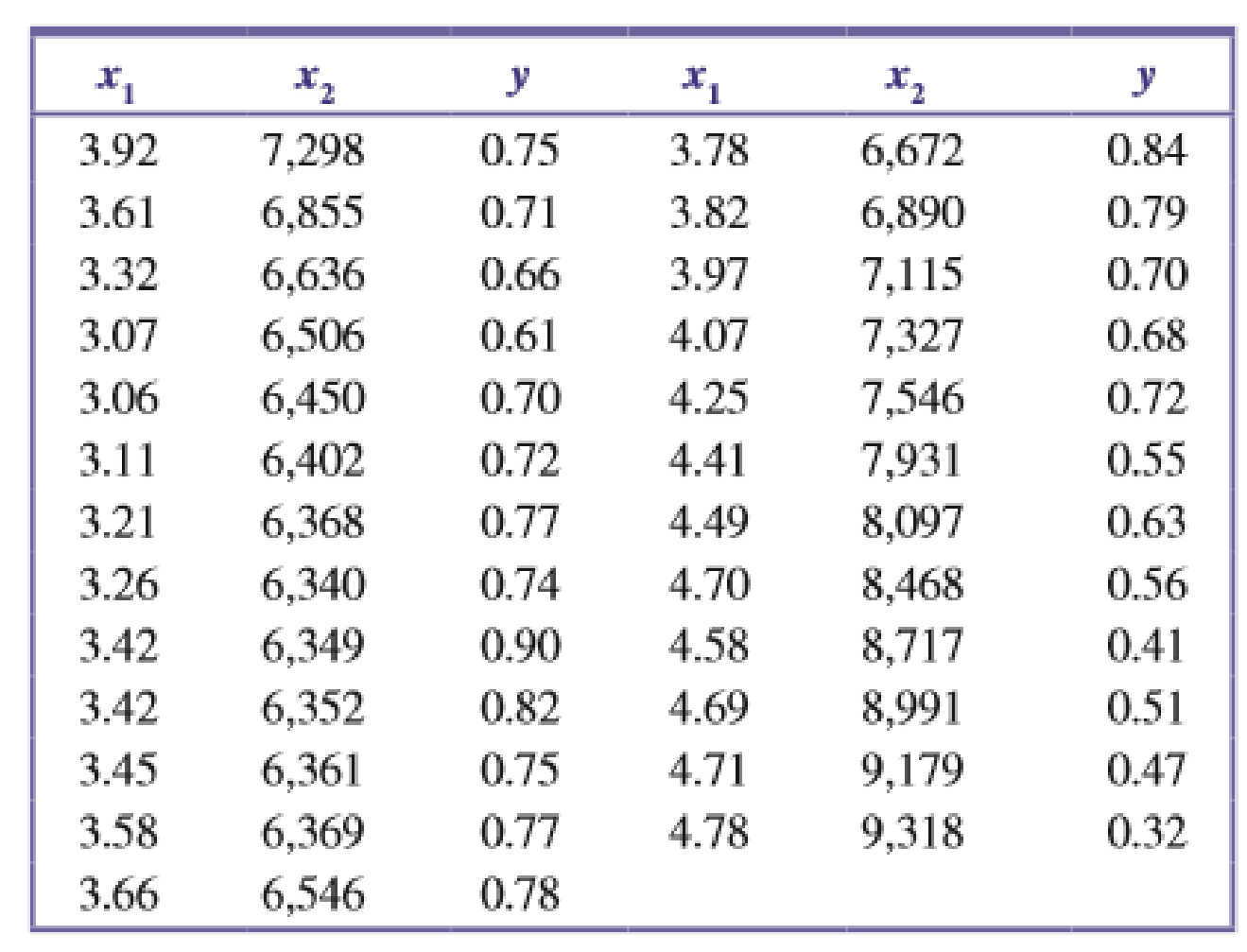
- a. Fit a multiple regression model using both independent variables.
- b. Use the F test to determine whether the model provides useful information for predicting profit margin.
- c. Interpret the values of R2 and se.
- d. Would a regression model using a single independent variable (x1 alone or x2 alone) have sufficed? Explain.
- e. Plot the (x1, x2) pairs. Does the plot indicate any sample observation that may have been highly influential in estimating the model coefficients? Explain. Do you see any evidence of multicollinearity? Explain.
Expert Solution & Answer
Want to see the full answer?
Check out a sample textbook solution
Students have asked these similar questions
a) Give a practical interpretation of the y-intercept of the regression line. b) What is the best-predicted value for the median hourly wage gain for the fifteenth year of schooling? c) The actual wage gain for the fifteenth year of schooling was 14%. How close was the predicted wage gain present to the actual value, i.e. what is the residual?
The November 24, 2001, issue of The Economist published economic data for 15
industrialized nations. Included were the percent changes in gross domestic product (GDP),
industrial production (IP), consumer prices (CP), and producer prices (PP) from Fall 2000
to Fall 2001, and the unemployment rate in Fall 2001 (UNEMP). An economist wants to
construct a model to predict GDP from the other variables. A fit of the model
GDP = , + P,IP + 0,UNEMP + f,CP + P,PP + €
yields the following output:
The regression equation is
GDP = 1.19 + 0.17 IP + 0.18 UNEMP + 0.18 CP – 0.18 PP
Predictor
Coef SE Coef
тР
Constant
1.18957 0.42180 2.82 0.018
IP
0.17326 0.041962 4.13 0.002
UNEMP
0.17918 0.045895 3.90 0.003
CP
0.17591 0.11365 1.55 0.153
PP
-0.18393 0.068808 -2.67 0.023
Predict the percent change in GDP for a country with IP = 0.5, UNEMP = 5.7, CP =
3.0, and PP = 4.1.
a.
b.
If two countries differ in unemployment rate by 1%, by how much would you predict
their percent changes in GDP to differ, other…
Q: The dataset posted below lists a sample of months and the advertising budget (in hundreds of dollars) for TV, radio and newspaper advertisements. Also included is whether a coupon was published for that month and the resulting sales (in thousands of dollars).
a) Develop a multiple regression model predicting the sales based off the four predictor variables: TV, radio, and newspaper advertising budget and whether a coupon is used. Recode Coupon as 0 = No and 1 = Yes. Report the estimated regression equation (Solve in Excel)
TV ($100)
radio ($100)
newspaper ($100)
Coupon
sales ($1000)
0.7
39.6
8.7
No
1.6
230.1
37.8
69.2
No
22.1
4.1
11.6
5.7
Yes
3.2
44.5
39.3
45.1
No
10.4
250.9
36.5
72.3
No
22.2
8.6
2.1
1
No
4.8
17.2
45.9
69.3
Yes
9.3
104.6
5.7
34.4
No
10.4
216.8
43.9
27.2
Yes
22.3
5.4
29.9
9.4
No
5.3
69
9.3
0.9
No
9.3
70.6
16
40.8
No
10.5
151.5
41.3
58.5
No
18.5
195.4
47.7
52.9
Yes
22.4
13.1
0.4
25.6
Yes
5.3
76.4
0.8…
Chapter 14 Solutions
Introduction To Statistics And Data Analysis
Ch. 14.1 - Prob. 1ECh. 14.1 - The authors of the paper Weight-Bearing Activity...Ch. 14.1 - Prob. 3ECh. 14.1 - Prob. 4ECh. 14.1 - Prob. 5ECh. 14.1 - Prob. 6ECh. 14.1 - Prob. 7ECh. 14.1 - Prob. 8ECh. 14.1 - Prob. 9ECh. 14.1 - The relationship between yield of maize (a type of...
Ch. 14.1 - Prob. 11ECh. 14.1 - A manufacturer of wood stoves collected data on y...Ch. 14.1 - Prob. 13ECh. 14.1 - Prob. 14ECh. 14.1 - Prob. 15ECh. 14.2 - Prob. 16ECh. 14.2 - State as much information as you can about the...Ch. 14.2 - Prob. 18ECh. 14.2 - Prob. 19ECh. 14.2 - Prob. 20ECh. 14.2 - The ability of ecologists to identify regions of...Ch. 14.2 - Prob. 22ECh. 14.2 - Prob. 23ECh. 14.2 - Prob. 24ECh. 14.2 - Prob. 25ECh. 14.2 - Prob. 26ECh. 14.2 - This exercise requires the use of a statistical...Ch. 14.2 - Prob. 28ECh. 14.2 - The article The Undrained Strength of Some Thawed...Ch. 14.2 - Prob. 30ECh. 14.2 - Prob. 31ECh. 14.2 - Prob. 32ECh. 14.2 - Prob. 33ECh. 14.2 - This exercise requires the use of a statistical...Ch. 14.2 - This exercise requires the use of a statistical...Ch. 14.3 - Prob. 36ECh. 14.3 - Prob. 37ECh. 14.3 - When Coastal power stations take in large amounts...Ch. 14.3 - Prob. 39ECh. 14.3 - The article first introduced in Exercise 14.28 of...Ch. 14.3 - Data from a random sample of 107 students taking a...Ch. 14.3 - Benevolence payments are monies collected by a...Ch. 14.3 - Prob. 43ECh. 14.3 - Prob. 44ECh. 14.3 - Prob. 45ECh. 14.3 - Prob. 46ECh. 14.3 - Exercise 14.26 gave data on fish weight, length,...Ch. 14.3 - Prob. 48ECh. 14.3 - Prob. 49ECh. 14.3 - Prob. 50ECh. 14.4 - Prob. 51ECh. 14.4 - Prob. 52ECh. 14.4 - The article The Analysis and Selection of...Ch. 14.4 - Prob. 54ECh. 14.4 - Prob. 55ECh. 14.4 - Prob. 57ECh. 14.4 - Prob. 58ECh. 14.4 - Prob. 59ECh. 14.4 - Prob. 60ECh. 14.4 - This exercise requires use of a statistical...Ch. 14.4 - Prob. 62ECh. 14 - Prob. 63CRCh. 14 - Prob. 64CRCh. 14 - The accompanying data on y = Glucose concentration...Ch. 14 - Much interest in management circles has focused on...Ch. 14 - Prob. 67CRCh. 14 - Prob. 68CRCh. 14 - Prob. 69CRCh. 14 - A study of pregnant grey seals resulted in n = 25...Ch. 14 - Prob. 71CRCh. 14 - Prob. 72CRCh. 14 - This exercise requires the use of a statistical...
Knowledge Booster


Learn more about
Need a deep-dive on the concept behind this application? Look no further. Learn more about this topic, statistics and related others by exploring similar questions and additional content below.Similar questions
- Find the equation of the regression line for the following data set. x 1 2 3 y 0 3 4arrow_forward1. Explain the purpose or use of the following:a. Linear regression equationb. Correlation coefficient.arrow_forwardA major brokerage company has an office in Miami, Florida. The manager of the office is evaluated based on the number of new clients generated each quarter. Data were collected that show the number of new customers added during each quarter between 2015 and 2018. A multiple regression model was developed with the number of new customers as the dependent and the following four independent variables: Period (1, …, 16): A variable that measures the trend; Q1 = 1 for first quarter, Q1 = 0 otherwise; Q2 = 1 for second quarter, Q2 = 0 otherwise; Q3 = 1 for third quarter, Q3 = 0 otherwise. Questions: 1. Explain each of the four slopes (Period, Q1, Q2, Q3). 2. How many new customers would you expect in the second quarter of the following year (2019)?arrow_forward
- An article in Technometrics by S. C. Narula and J. F. Wellington (“Prediction, Linear Regression, and a Minimum Sum of Relative Errors,” Vol. 19, 1977) presents data on the selling price (y) and annual taxes (x) for 24 houses. The taxes include local, school and county taxes. The data are shown in the following table. Sale Price/1000 Taxes/1000 25.9 4.9176 29.5 5.0208 27.9 4.5429 25.9 4.5573 29.9 5.0597 29.9 3.8910 30.9 5.8980 28.9 5.6039 35.9 5.8282 31.5 5.3003 31.0 6.2712 30.9 5.9592 30.0 5.0500 36.9 8.2464 41.9 6.6969 40.5 7.7841 43.9 9.0384 37.5 5.9894 37.9 7.5422 44.5 8.7951 37.9 6.0831 38.9 8.3607 36.9 8.1400…arrow_forwardThe county assessor is studying housing demand and is interested in developing a regression model to estimate the market value (i.e., selling price) of residential property within her jurisdiction. The assessor suspects that the most important variable affecting selling price (measured in thousands of dollars) is the size of house (measured in hundreds of square feet). She randomly selects 15 houses and measures both the selling price and size, as shown in the following table. Complete the table and then use it to determine the estimated regression line. Observation i 1 2 3 4 5 6 7 8 9 10 i 11 12 13 14 15 Total O 8.074 Regression Parameters Slope (B) Intercept (α) 10.181 8.358 O 0.327 Size (x 100 sq. ft.) O 0.316 12 20.2 27 O 0.398 30 30 O Yes 21.4 21.6 25.2 37.2 14.4 15 22.4 23.9 26.6 30.7 357.60 O No What is the standard error of the estimate (Se)? In words, for each hundred square feet, the expected selling price of a house Selling Price (x $1,000) Ii Yi y 265.2 253.4 12 2 20.2…arrow_forwardThe county assessor is studying housing demand and is interested in developing a regression model to estimate the market value (i.e., selling price) of residential property within his jurisdiction. The assessor suspects that the most important variable affecting selling price (measured in thousands of dollars) is the size of house (measured in hundreds of square feet). He randomly selects 15 houses and measures both the selling price and size, as shown in the following table. Complete the table and then use it to determine the estimated regression line. Observation Size Selling Price (x 100 sq. ft.) (x $1,000) ii xixi yiyi xixiyiyi xi2xi2 yi2yi2 1 12 265.2 3,182.40 144.00 70,331.04 2 20.2 279.6 5,647.92 408.04 78,176.16 3 27 311.2 8,402.40 729.00 96,845.44 4 30 328.0 9,840.00 900.00 107,584.00 5 30 352.0 10,560.00 900.00 123,904.00 6 21.4 281.2 6,017.68 457.96 79,073.44 7 21.6 288.4 6,229.44 466.56 83,174.56 8 25.2 292.8 7,378.56 635.04…arrow_forward
- Please use the accompanying Excel data set or accompanying Text file data set when completing the following exercise. An article in Technometrics by S. C. Narula and J. F. Wellington ("Prediction, Linear Regression, and a Minimum Sum of Relative Errors," Vol. 19, 1977) presents data on the selling price (y) and annual taxes (x) for 24 houses. The taxes include local, school and county taxes. The data are shown in the following table. Sale Price/1000 Taxes/1000 25.9 4.9176 29.5 5.0208 27.9 4.5429 25.9 4.5573 29.9 5.0597 29.9 3.8910 30.9 5.8980 28.9 5.6039 35.9 5.8282 31.5 5.3003 31.0 6.2712 30.9 5.9592 30.0 5.0500 36.9 8.2464 41.9 6.6969 40.5 7.7841 43.9 9.0384 37.5 5.9894 37.9 7.5422 44.5 8.7951 37.9 6.0831 38.9 8.3607arrow_forward2arrow_forwardThe use of multiple logistic regression is warranted when there are two or more independent quantitative or nominal variables and one dichotomous dependent variable. a. True b. Falsearrow_forward
- 1a)Use regression analysis to investigate the relationship between the number of fatal accidents and the percentage of drivers under the age of 21. 1b)What conclusion and recommendations can you derive from your analysis?arrow_forwardThe U.S. Postal Service is attempting to reduce the number of complaints made by the public against its workers. To facilitate this task, a staff analyst for the service regresses the number of complaints lodged against an employee last year on the hourly wage of the employee for the year. The analyst ran a simple linear regression in SPSS. The results are shown below. The current minimum wage is $5.15. If an employee earns the minimum wage, how many complaints can that employee expect to receive? Is the regression coefficient statistically significant? How can you tell?arrow_forwardThe accompanying table shows the percentage of employment in STEM (science, technology, engineering, and math) occupations and mean annual wage (in thousands of dollars) for 1616 industries. The equation of the regression line is ModifyingAbove y with caret equals=1.125x+46.695. Use these data to construct a 90% prediction interval for the mean annual wage (in thousands of dollars) when the percentage of employment in STEM occupations is 12% in the industry. Interpret this interval. Construct a 90% prediction interval for the mean annual wage (in thousands of dollars) when the percentage of employment in STEM occupations is 12% in the industry. nothingless than<yless than<nothing (Round to three decimal places as needed.) Interpret the prediction interval. Select the correct choice below and fill in the answer boxes to complete your choice. (Round to the nearest whole number as needed.) A. One can be 90% confident that the mean annual wage will…arrow_forward
arrow_back_ios
SEE MORE QUESTIONS
arrow_forward_ios
Recommended textbooks for you
 Linear Algebra: A Modern IntroductionAlgebraISBN:9781285463247Author:David PoolePublisher:Cengage Learning
 Functions and Change: A Modeling Approach to Coll...AlgebraISBN:9781337111348Author:Bruce Crauder, Benny Evans, Alan NoellPublisher:Cengage Learning
 Big Ideas Math A Bridge To Success Algebra 1: Stu...AlgebraISBN:9781680331141Author:HOUGHTON MIFFLIN HARCOURTPublisher:Houghton Mifflin Harcourt
Linear Algebra: A Modern Introduction
Algebra
ISBN:9781285463247
Author:David Poole
Publisher:Cengage Learning
Functions and Change: A Modeling Approach to Coll...
Algebra
ISBN:9781337111348
Author:Bruce Crauder, Benny Evans, Alan Noell
Publisher:Cengage Learning
Big Ideas Math A Bridge To Success Algebra 1: Stu...
Algebra
ISBN:9781680331141
Author:HOUGHTON MIFFLIN HARCOURT
Publisher:Houghton Mifflin Harcourt
Correlation Vs Regression: Difference Between them with definition & Comparison Chart; Author: Key Differences;https://www.youtube.com/watch?v=Ou2QGSJVd0U;License: Standard YouTube License, CC-BY
Correlation and Regression: Concepts with Illustrative examples; Author: LEARN & APPLY : Lean and Six Sigma;https://www.youtube.com/watch?v=xTpHD5WLuoA;License: Standard YouTube License, CC-BY