
Introduction To Statistics And Data Analysis
6th Edition
ISBN: 9781337793612
Author: PECK, Roxy.
Publisher: Cengage Learning,
expand_more
expand_more
format_list_bulleted
Concept explainers
Videos
Textbook Question
Chapter 14, Problem 65CR
The accompanying data on y = Glucose concentration (g/L) and x = Fermentation lime (days) for a particular blend of malt liquor were read from a
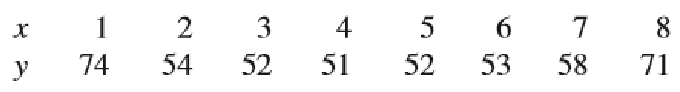
- a. Construct a scatterplot for these data. Based on the scatterplot, what type of model would you suggest?
- b. Minitab output resulting from fitting a multiple regression model with x1 = x and x2 = x2 is shown here. Does this quadratic model specify a useful relationship between y and x?
The regression equation is
Y = 84.5 − 15.9X1 + 1.77X2
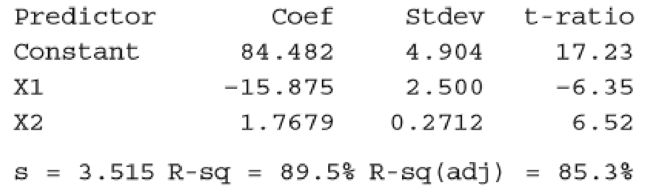
- c. Could the quadratic term be eliminated? That is, would a simple linear model have sufficed? Test using a 0.05 significance level.
Expert Solution & Answer
Want to see the full answer?
Check out a sample textbook solution
Students have asked these similar questions
The article "Lead Dissolution from Lead Smelter Slags Using Magnesium Chloride
Solutions" (A. Xenidis, T. Lillis, and I. Hallikia, The AusIMM Proceedings, 1999:37-14)
discusses an investigation of leaching rates of lead in solutions of magnesium chloride. The
data in the following table (read from a graph) present the percentage of lead that has been
extracted at various times (in minutes).
Time (t)
4 8 16 30 60 120
Percent extracted (v) |1.2 1.6 2.3 2.8 3.6 4.4
a. The article suggests fitting a quadratic model y = Bo + B,t + Bz² + ɛ to these data. Fit
this model, and compute the standard deviations of the coefficients.
b. The reaction rate at time t is given by the derivative dy/dt = B, + 2B,t. Estimate the
time at which the reaction rate will be equal to 0.05.
c. The reaction rate at t = Oisequal to B1. Find a 95% confidence interval for the reaction
rate at t = 0.
d. Can you conclude that the reaction rate is decreasing with time? Explain.
Consider the forecasting model with a simple, linear trend:
It = ß1 + Bzt + et
Where t is the index for t = 1, 2, ..., T. The OLS estimator of B1, B2 is:
E (4t – Ht)(t – t)
B2 =
Bi = y – Bạf
Where "bars" standards for the sample mean e.g. t = E-1 Yt.
a Using those formulas, derive the OLS estimator of the regression yt = a1+a2(t – 1) + Et. Compare to
Bị and B2.
81 + 82t + ɛt.
b Again, using those formulas, derive the OLS estimator of the regression Yt/1000
Compare to B1 and B2.
5.1 Application: Yo.
e
Here is data for the amount of fat (in grams) for McDonald's chicken sandwiches:
Sandwich
McChicken Ⓒ
Premium Grilled Chicken Classic Sandwich
Premium Crispy Chicken Classic Sandwich
Premium Grilled Chicken Club Sandwich
Premium Crispy Chicken Club Sandwich
Premium Grilled Chicken Ranch BLT Sandwich
Premium Crispy Chicken Ranch BLT Sandwich
Southern Style Crispy Chicken Sandwich
Ranch Snack Wrap (Crispy)
Ranch Snack Wrap (Grilled)
Honey Mustard Snack Wrap (Crispy).
Honey Mustard Snack Wrap (Grilled)
Chipotle BBQ Snack Wrap (Crispy)
Chipotle BBQ Snack Wrap (Grilled)
Find the median and IQR.
M = type your answer...
IQR= type your answer...
C
54
do 5
%
Fat
16 g
10 g
20 g
17 g
28 g
12 g
23 g
17 g
17 g
10 g
16 g
99
15 g
99
A
6
g
g
DELL
&
7
O
8
O
(
9
%
)
0
Chapter 14 Solutions
Introduction To Statistics And Data Analysis
Ch. 14.1 - Prob. 1ECh. 14.1 - The authors of the paper Weight-Bearing Activity...Ch. 14.1 - Prob. 3ECh. 14.1 - Prob. 4ECh. 14.1 - Prob. 5ECh. 14.1 - Prob. 6ECh. 14.1 - Prob. 7ECh. 14.1 - Prob. 8ECh. 14.1 - Prob. 9ECh. 14.1 - The relationship between yield of maize (a type of...
Ch. 14.1 - Prob. 11ECh. 14.1 - A manufacturer of wood stoves collected data on y...Ch. 14.1 - Prob. 13ECh. 14.1 - Prob. 14ECh. 14.1 - Prob. 15ECh. 14.2 - Prob. 16ECh. 14.2 - State as much information as you can about the...Ch. 14.2 - Prob. 18ECh. 14.2 - Prob. 19ECh. 14.2 - Prob. 20ECh. 14.2 - The ability of ecologists to identify regions of...Ch. 14.2 - Prob. 22ECh. 14.2 - Prob. 23ECh. 14.2 - Prob. 24ECh. 14.2 - Prob. 25ECh. 14.2 - Prob. 26ECh. 14.2 - This exercise requires the use of a statistical...Ch. 14.2 - Prob. 28ECh. 14.2 - The article The Undrained Strength of Some Thawed...Ch. 14.2 - Prob. 30ECh. 14.2 - Prob. 31ECh. 14.2 - Prob. 32ECh. 14.2 - Prob. 33ECh. 14.2 - This exercise requires the use of a statistical...Ch. 14.2 - This exercise requires the use of a statistical...Ch. 14.3 - Prob. 36ECh. 14.3 - Prob. 37ECh. 14.3 - When Coastal power stations take in large amounts...Ch. 14.3 - Prob. 39ECh. 14.3 - The article first introduced in Exercise 14.28 of...Ch. 14.3 - Data from a random sample of 107 students taking a...Ch. 14.3 - Benevolence payments are monies collected by a...Ch. 14.3 - Prob. 43ECh. 14.3 - Prob. 44ECh. 14.3 - Prob. 45ECh. 14.3 - Prob. 46ECh. 14.3 - Exercise 14.26 gave data on fish weight, length,...Ch. 14.3 - Prob. 48ECh. 14.3 - Prob. 49ECh. 14.3 - Prob. 50ECh. 14.4 - Prob. 51ECh. 14.4 - Prob. 52ECh. 14.4 - The article The Analysis and Selection of...Ch. 14.4 - Prob. 54ECh. 14.4 - Prob. 55ECh. 14.4 - Prob. 57ECh. 14.4 - Prob. 58ECh. 14.4 - Prob. 59ECh. 14.4 - Prob. 60ECh. 14.4 - This exercise requires use of a statistical...Ch. 14.4 - Prob. 62ECh. 14 - Prob. 63CRCh. 14 - Prob. 64CRCh. 14 - The accompanying data on y = Glucose concentration...Ch. 14 - Much interest in management circles has focused on...Ch. 14 - Prob. 67CRCh. 14 - Prob. 68CRCh. 14 - Prob. 69CRCh. 14 - A study of pregnant grey seals resulted in n = 25...Ch. 14 - Prob. 71CRCh. 14 - Prob. 72CRCh. 14 - This exercise requires the use of a statistical...
Knowledge Booster


Learn more about
Need a deep-dive on the concept behind this application? Look no further. Learn more about this topic, statistics and related others by exploring similar questions and additional content below.Similar questions
- For the following table of data. x 1 2 3 4 5 6 7 8 9 10 y 0 0.5 1 2 2.5 3 3 4 4.5 5 a. draw a scatterplot. b. calculate the correlation coefficient. c. calculate the least squares line and graph it on the scatterplot. d. predict the y value when x is 11.arrow_forwardUrban Travel Times Population of cities and driving times are related, as shown in the accompanying table, which shows the 1960 population N, in thousands, for several cities, together with the average time T, in minutes, sent by residents driving to work. City Population N Driving time T Los Angeles 6489 16.8 Pittsburgh 1804 12.6 Washington 1808 14.3 Hutchinson 38 6.1 Nashville 347 10.8 Tallahassee 48 7.3 An analysis of these data, along with data from 17 other cities in the United States and Canada, led to a power model of average driving time as a function of population. a Construct a power model of driving time in minutes as a function of population measured in thousands b Is average driving time in Pittsburgh more or less than would be expected from its population? c If you wish to move to a smaller city to reduce your average driving time to work by 25, how much smaller should the city be?arrow_forwardAn article in the Fire Safety Journal (“The Effect of Nozzle Design on the Stability and Performance of Turbulent Water Jets,” Vol. 4, August 1981) describes an experiment in which a shape factor was determined for several different nozzle designs at six levels of jet efflux velocity. Interest focused on potential differences between nozzle designs (blocks), with velocity considered as a nuisance variable. The data are shown below: Jet Efflux Velocity (m/s) Nozzle Design 11.73 14.37 16.59 20.43 23.46 28.74 1 0.78 0.80 0.81 0.75 0.77 0.78 2 0.85 0.85 0.92 0.86 0.81 0.83 3 0.93 0.92 0.95 0.89 0.89 0.83 4 1.14 0.97 0.98 0.88 0.86 0.83 5 0.97 0.86 0.78 0.76 0.76 0.75 1) Write the null hypothesis and the alternative hypothesis (for the factor). 2) Find the ANOVA table. (round to five decimal places). 3) What is your decision about the null hypothesis, consider ?. 4) If your decision in part (4) was reject , perform Tukey test to determine which pairwise means are…arrow_forward
- Is it possible to get the following from a set of experimental data: (a) r23 = 0.8, r13 = - 0.5, r12 = 0.6 %3D %3D %3D (b) r23 = 0.7, r13 = - 0.4, r12 = 0.6 %3D %3D %3Darrow_forwardData from the US Department of Energy’s US Energy Information Administration (eia.doe.gov) provides a look at the energy-related carbon dioxide emissions by end use sector (residential, commercial, industrial, transportation) from years 1990 to 2009. (Report # DOE/EIA0573(2009)). Here we would like to see if the CO2 emissions from the Industrial sector are less than that from the Transportation sector. Below are the results: 14. What type of study is this? a. Paired b. Two-Sample Independent 15. What type of plot would we use? a. Histogram of the differences b. Side-by-side boxplots c. Pie chart d. Bar graph 16. Was the HOV/pooled test used above (hint: look at the df)? YES NO 17. Is there evidence that the CO2 emissions from the Industrial sector are less than that from the Transportation sector? YES NO 18. If we were to test to see if there was a difference between the CO2 emissions from the Industrial sector and the Transportation sector, what would be the p-value? (report to 3…arrow_forwardThe output of a solar panel (photovoltaic) system depends on its size. A manufacturer states that the average daily production of its 1.5 kW system is 6.6 kilowatt hours (kWh) for Perth conditions. A consumer group monitored this 1.5 kW system in 20 different Perth homes and measured the average daily production by the systems in these homes over a one month period during October. The data is provided here. kWh 6.2, 5.8, 5.9, 6.1, 6.4, 6.3, 6.9, 5.5, 7.4, 6.7, 6.3, 6.2, 7.1, 6.8, 5.9, 5.4, 7.2, 6.7, 5.8, 6.9 1. Analyse the consumer group’s data to test if the manufacturer’s claim of an average of 6.6 kWh per day is reasonable. State appropriate hypotheses, assumptions and decision rule at α = 0.10. What conclusions would you report to the consumer group? (Hint: You will need to find Descriptive Statistics first.) 2. If 48 homes in the central Australian city of Alice Springs had this system installed and similar data was collected, in order to assess whether average daily production in…arrow_forward
- Apply the predictive control law to a fifth-order process:Y(s)/(s)=1/(5s+1)⁵.Evaluate the effect of tuning paramete rJ on the set-pointresponses for values of J=3, 4, 6, and 8 and Δt=5 min.arrow_forwardThe article "Characteristics and Trends of River Discharge into Hudson, James, and Ungava Bays, 1964-2000" (S. Dery, M. Stieglitz, et al., Journal of Climate, 2005:2540-2557) presents measurements of discharge rate x (in kmlyr) andpeakflow y (in m/s) for 42 rivers that drain into the Hudson, James, and Ungava Bays. The data are shown in the following table: Discharge Peak Flow 94.24 4110.3 66.57 4961.7 59.79 10275.5 48.52 6616.9 40.00 7459.5 32.30 2784.4 31.20 3266.7 30.69 4368.7 26.65 1328.5 22.75 4437.6 21.20 1983.0 20.57 1320.1 19.77 1735.7 18.62 1944.1 17.96 3420.2 17.84 2655.3 16.06 3470.3 1561.6 14.69 11.63 869.8 11.19 936.8 11.08 1315.7 10.92 1727.1 9.94 768.1 7.86 483.3arrow_forwardAn environmental group took a sample from a river under study to check on the biochemical oxygen demand (BOD) of the organisms living in the river. The BOD test was conducted over a period of time (in days). The resulting data follow: Time (days): 1 2 4 6 8 10 12 14 18 20 BOD (mg/liter) 0.6 0.7 1.5 1.9 2.1 2.6 2.9 3.7 3.7 3.8 23 16 3.5arrow_forward
arrow_back_ios
arrow_forward_ios
Recommended textbooks for you
 Calculus For The Life SciencesCalculusISBN:9780321964038Author:GREENWELL, Raymond N., RITCHEY, Nathan P., Lial, Margaret L.Publisher:Pearson Addison Wesley,
 Functions and Change: A Modeling Approach to Coll...AlgebraISBN:9781337111348Author:Bruce Crauder, Benny Evans, Alan NoellPublisher:Cengage Learning
 Linear Algebra: A Modern IntroductionAlgebraISBN:9781285463247Author:David PoolePublisher:Cengage Learning
 Glencoe Algebra 1, Student Edition, 9780079039897...AlgebraISBN:9780079039897Author:CarterPublisher:McGraw Hill
Calculus For The Life Sciences
Calculus
ISBN:9780321964038
Author:GREENWELL, Raymond N., RITCHEY, Nathan P., Lial, Margaret L.
Publisher:Pearson Addison Wesley,
Functions and Change: A Modeling Approach to Coll...
Algebra
ISBN:9781337111348
Author:Bruce Crauder, Benny Evans, Alan Noell
Publisher:Cengage Learning
Linear Algebra: A Modern Introduction
Algebra
ISBN:9781285463247
Author:David Poole
Publisher:Cengage Learning
Glencoe Algebra 1, Student Edition, 9780079039897...
Algebra
ISBN:9780079039897
Author:Carter
Publisher:McGraw Hill
Correlation Vs Regression: Difference Between them with definition & Comparison Chart; Author: Key Differences;https://www.youtube.com/watch?v=Ou2QGSJVd0U;License: Standard YouTube License, CC-BY
Correlation and Regression: Concepts with Illustrative examples; Author: LEARN & APPLY : Lean and Six Sigma;https://www.youtube.com/watch?v=xTpHD5WLuoA;License: Standard YouTube License, CC-BY