PRACTICE OF STATISTICS F/AP EXAM
6th Edition
ISBN: 9781319113339
Author: Starnes
Publisher: MAC HIGHER
bartleby

Videos

Question
Book Icon
Chapter 12.2, Problem 48E

(a)

To determine

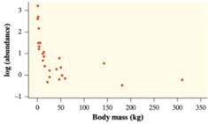
To Explain: the better relationship between abundance and body mass.

(a)

Expert Solution
Check Mark

Answer to Problem 48E

Power model

Explanation of Solution

Given:

  PRACTICE OF STATISTICS F/AP EXAM, Chapter 12.2, Problem 48E , additional homework tip  1

  PRACTICE OF STATISTICS F/AP EXAM, Chapter 12.2, Problem 48E , additional homework tip  2

  PRACTICE OF STATISTICS F/AP EXAM, Chapter 12.2, Problem 48E , additional homework tip  3

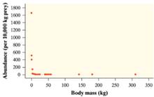
It is observed that the given scatter plot between log(abundance) and log(body mass). is not having strong curvature and therefore it would be appropriate to utilize a linear model between the two variables of the scatter plot. Therefore it is appropriate to utilize a linear model between log(abundance) and log(body mass).

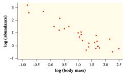
General linear model to expect log(abundance) and log(body mass).

  log(abundance)=a+b(body mass)

Taking the exponential

  abundance=elog(abundance)=ea+b(body mass)=eaeb(body mass)

Therefore the model associate with the model abundance=eaeb(body mass) .It is power model between abundance and body mass. Although the linear model between abundance and log(body mass) is appropriate, the power model between abundance and body mass is also appropriate.

(b)

To determine

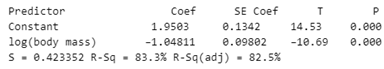
To find: the equation of the least-squares regression line on the basis of given computer output.

(b)

Expert Solution
Check Mark

Answer to Problem 48E

  logy=1.95031.04811logx

Explanation of Solution

Given:

  PRACTICE OF STATISTICS F/AP EXAM, Chapter 12.2, Problem 48E , additional homework tip  4

Calculation:

General equation for the least square regression line

  y^=b0+b1x

The calculated of the constant b0 is mention in the row “constant” and in the column “Coef” of the output of the computer

  b0 =1.9503

The calculated of the slope b1 is mention in the row “Distance” and in the column “Coef” of the output of the computer

  b1 =-1.04811

Putting the value of b0 and b1

  y^=b0+b1xy^=1.95031.04811x

Taking the logarithm

  logy=1.95031.04811logx

Where x is representing the body mass and y is representing the abundance.

(c)

To determine

To Explain: the prediction of the abundance of black bears on the basis of part (b).

(c)

Expert Solution
Check Mark

Answer to Problem 48E

0.775532 per 10000kg prey

Explanation of Solution

Given:

  PRACTICE OF STATISTICS F/AP EXAM, Chapter 12.2, Problem 48E , additional homework tip  5

Calculation:

From the part (b)

  logy=1.95031.04811logx

Where x is representing the body mass and y is representing the abundance.

Putting the value of x into the equation

  logy=1.95031.04811logxlogy=1.95031.04811log(92.5)logy=0.1104

Taking the exponential

  y^=10logy=100.1104=0.775532

Therefore the expected abundance is 0.775532 per 10000kg prey

(d)

To determine

To Calculate: here is given linear regression in part (b), is it expected that prediction in part (c) to be too large, too small or about right, justify the answer.

(d)

Expert Solution
Check Mark

Answer to Problem 48E

About right

Explanation of Solution

Given:

  PRACTICE OF STATISTICS F/AP EXAM, Chapter 12.2, Problem 48E , additional homework tip  6

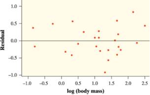
From the part (c) it is prediction for the body mass of 92.5 kilogram.

  log(92.5)=1.966142

In the residual figure, it is observed that the dots between 1.5 and 2.0 are both below and above the horizontal line at 0. Moreover it is noticed that the horizontal line 0 lies in the mid between these dots and therefore it is expected that prediction at about 2 to be about right.

Chapter 12 Solutions

PRACTICE OF STATISTICS F/AP EXAM

Ch. 12.1 - Prob. 11ECh. 12.1 - Prob. 12ECh. 12.1 - Prob. 13ECh. 12.1 - Prob. 14ECh. 12.1 - Prob. 15ECh. 12.1 - Prob. 16ECh. 12.1 - Prob. 17ECh. 12.1 - Prob. 18ECh. 12.1 - Prob. 19ECh. 12.1 - Prob. 20ECh. 12.1 - Prob. 21ECh. 12.1 - Prob. 22ECh. 12.1 - Prob. 23ECh. 12.1 - Prob. 24ECh. 12.1 - Prob. 25ECh. 12.1 - Prob. 26ECh. 12.1 - Prob. 27ECh. 12.1 - Prob. 28ECh. 12.1 - Prob. 29ECh. 12.1 - Prob. 30ECh. 12.1 - Prob. 31ECh. 12.1 - Prob. 32ECh. 12.2 - Prob. 33ECh. 12.2 - Prob. 34ECh. 12.2 - Prob. 35ECh. 12.2 - Prob. 36ECh. 12.2 - Prob. 37ECh. 12.2 - Prob. 38ECh. 12.2 - Prob. 39ECh. 12.2 - Prob. 40ECh. 12.2 - Prob. 41ECh. 12.2 - Prob. 42ECh. 12.2 - Prob. 43ECh. 12.2 - Prob. 44ECh. 12.2 - Prob. 45ECh. 12.2 - Prob. 46ECh. 12.2 - Prob. 47ECh. 12.2 - Prob. 48ECh. 12.2 - Prob. 49ECh. 12.2 - Prob. 50ECh. 12.2 - Prob. 51ECh. 12.2 - Prob. 52ECh. 12.2 - Prob. 53ECh. 12.2 - Prob. 54ECh. 12.2 - Prob. 55ECh. 12.2 - Prob. 56ECh. 12.2 - Prob. 57ECh. 12.2 - Prob. 58ECh. 12 - Prob. R12.1RECh. 12 - Prob. R12.2RECh. 12 - Prob. R12.3RECh. 12 - Prob. R12.4RECh. 12 - Prob. R12.5RECh. 12 - Prob. R12.6RECh. 12 - Prob. T12.1SPTCh. 12 - Prob. T12.2SPTCh. 12 - Prob. T12.3SPTCh. 12 - Prob. T12.4SPTCh. 12 - Prob. T12.5SPTCh. 12 - Prob. T12.6SPTCh. 12 - Prob. T12.7SPTCh. 12 - Prob. T12.8SPTCh. 12 - Prob. T12.9SPTCh. 12 - Prob. T12.10SPTCh. 12 - Prob. T12.11SPTCh. 12 - Prob. T12.12SPTCh. 12 - Prob. AP4.1CPTCh. 12 - Prob. AP4.2CPTCh. 12 - Prob. AP4.3CPTCh. 12 - Prob. AP4.4CPTCh. 12 - Prob. AP4.5CPTCh. 12 - Prob. AP4.6CPTCh. 12 - Prob. AP4.7CPTCh. 12 - Prob. AP4.8CPTCh. 12 - Prob. AP4.9CPTCh. 12 - Prob. AP4.10CPTCh. 12 - Prob. AP4.11CPTCh. 12 - Prob. AP4.12CPTCh. 12 - Prob. AP4.13CPTCh. 12 - Prob. AP4.14CPTCh. 12 - Prob. AP4.15CPTCh. 12 - Prob. AP4.16CPTCh. 12 - Prob. AP4.17CPTCh. 12 - Prob. AP4.18CPTCh. 12 - Prob. AP4.19CPTCh. 12 - Prob. AP4.20CPTCh. 12 - Prob. AP4.21CPTCh. 12 - Prob. AP4.22CPTCh. 12 - Prob. AP4.23CPTCh. 12 - Prob. AP4.24CPTCh. 12 - Prob. AP4.25CPTCh. 12 - Prob. AP4.26CPTCh. 12 - Prob. AP4.27CPTCh. 12 - Prob. AP4.28CPTCh. 12 - Prob. AP4.29CPTCh. 12 - Prob. AP4.30CPTCh. 12 - Prob. AP4.31CPTCh. 12 - Prob. AP4.32CPTCh. 12 - Prob. AP4.33CPTCh. 12 - Prob. AP4.34CPTCh. 12 - Prob. AP4.35CPTCh. 12 - Prob. AP4.36CPTCh. 12 - Prob. AP4.37CPTCh. 12 - Prob. AP4.38CPTCh. 12 - Prob. AP4.39CPTCh. 12 - Prob. AP4.40CPTCh. 12 - Prob. AP4.41CPTCh. 12 - Prob. AP4.42CPTCh. 12 - Prob. AP4.43CPTCh. 12 - Prob. AP4.44CPTCh. 12 - Prob. AP4.45CPTCh. 12 - Prob. AP4.46CPT
Knowledge Booster
Background pattern image
Statistics
Learn more about
Need a deep-dive on the concept behind this application? Look no further. Learn more about this topic, statistics and related others by exploring similar questions and additional content below.
Recommended textbooks for you
Text book image
MATLAB: An Introduction with Applications
Statistics
ISBN:9781119256830
Author:Amos Gilat
Publisher:John Wiley & Sons Inc
Text book image
Probability and Statistics for Engineering and th...
Statistics
ISBN:9781305251809
Author:Jay L. Devore
Publisher:Cengage Learning
Text book image
Statistics for The Behavioral Sciences (MindTap C...
Statistics
ISBN:9781305504912
Author:Frederick J Gravetter, Larry B. Wallnau
Publisher:Cengage Learning
Text book image
Elementary Statistics: Picturing the World (7th E...
Statistics
ISBN:9780134683416
Author:Ron Larson, Betsy Farber
Publisher:PEARSON
Text book image
The Basic Practice of Statistics
Statistics
ISBN:9781319042578
Author:David S. Moore, William I. Notz, Michael A. Fligner
Publisher:W. H. Freeman
Text book image
Introduction to the Practice of Statistics
Statistics
ISBN:9781319013387
Author:David S. Moore, George P. McCabe, Bruce A. Craig
Publisher:W. H. Freeman
Hypothesis Testing using Confidence Interval Approach; Author: BUM2413 Applied Statistics UMP;https://www.youtube.com/watch?v=Hq1l3e9pLyY;License: Standard YouTube License, CC-BY
Hypothesis Testing - Difference of Two Means - Student's -Distribution & Normal Distribution; Author: The Organic Chemistry Tutor;https://www.youtube.com/watch?v=UcZwyzwWU7o;License: Standard Youtube License