
Introductory Statistics (10th Edition)
10th Edition
ISBN: 9780321989178
Author: Neil A. Weiss
Publisher: PEARSON
expand_more
expand_more
format_list_bulleted
Videos
Textbook Question
Chapter 15.3, Problem 93E
In Exercises 15.92–15.97, presume that the assumptions for regression inferences are met.
15.93 Corvette Prices. Following are the age and price data for Corvettes from Exercise 15.23.
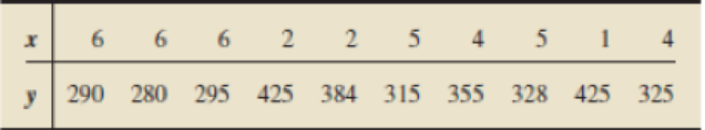
- a. Obtain a point estimate for the
mean price of all 4-year-old Corvettes. - b. Determine a 90% confidence interval for the mean price of all 4-ycar-old Corvettes.
- c. Find the predicted price of a 4-year-old Corvette.
- d. Determine a 90% prediction interval for the price of a 4-ycar-old Corvette.
- e. Draw graphs similar to those in Fig. 15.11 on page 683, showing both the 90% confidence interval from part (b) and the 90% prediction interval from part (d).
- f. Why is the prediction interval wider than the confidence interval?
Expert Solution & Answer
Want to see the full answer?
Check out a sample textbook solution
Students have asked these similar questions
a. Develop an estimated regression equation that can be used to predict annual sales given the years of experience. Use the excel regression tool.
b. Use the estimated regression equation to predict annual sales for a salesperson with 9 years of experience. Provide an approximate 95% confidence interval.
The table below lists weights (carats) and prices (dollars) of randomly selected diamonds. Find the (a) explained variation, (b) unexplained variation, and (c) indicated prediction interval. There is sufficient
evidence to support a claim of a linear correlation, so it is reasonable to use regression equation when making predictions. For the prediction interval, use a 95% confidence level with a diamond that
weighs 0.8 carats.
Weight
Price
a. Find the explained variation.
0.3
$500
(Round to the nearest whole number as needed.)
0.4
$1165
0.5
$1350
G
0.5
$1404
1.0
$5655
0.7
$2283
Q
A survey conducted by a research team was to investigate how the education level, tenure in current employment, and age, are related to annual income. A sample 20 emloyees is selected and the data is given below.
1. Which variable has significant relationship with income at 0.05 level of significance?
Chapter 15 Solutions
Introductory Statistics (10th Edition)
Ch. 15.1 - Suppose that x and y are predictor and response...Ch. 15.1 - Prob. 2ECh. 15.1 - Prob. 3ECh. 15.1 - Prob. 4ECh. 15.1 - Prob. 5ECh. 15.1 - In Exercises 15.315.6, assume that the variables...Ch. 15.1 - The difference between an observed value and a...Ch. 15.1 - Identify two graphs used in a residual analysis to...Ch. 15.1 - Which graph used in a residual analysis provides...Ch. 15.1 - Figure 15.8 shows three residual plots and a...
Ch. 15.1 - Figure 15.9 on the next page shows three residual...Ch. 15.1 - In Exercises 15.1215.21, we repeat the data and...Ch. 15.1 - In Exercises 15.1215.21, we repeat the data and...Ch. 15.1 - Prob. 14ECh. 15.1 - Prob. 15ECh. 15.1 - Prob. 16ECh. 15.1 - Prob. 17ECh. 15.1 - Prob. 18ECh. 15.1 - Prob. 19ECh. 15.1 - Prob. 20ECh. 15.1 - Prob. 21ECh. 15.1 - Prob. 22ECh. 15.1 - Prob. 23ECh. 15.1 - Prob. 24ECh. 15.1 - Prob. 25ECh. 15.1 - In Exercises 15.2215.27, we repeat the information...Ch. 15.1 - Prob. 27ECh. 15.1 - Prob. 28ECh. 15.1 - In Exercises 15.2815.33, a. compute the standard...Ch. 15.1 - Prob. 30ECh. 15.1 - In Exercises 15.2815.33, a. compute the standard...Ch. 15.1 - In Exercises 15.2815.33, a. compute the standard...Ch. 15.1 - In Exercises 15.2815.33, a. compute the standard...Ch. 15.1 - In Exercises 15.3415.43, use the technology of...Ch. 15.1 - In Exercises 15.3415.43, use the technology of...Ch. 15.1 - In Exercises 15.3415.43, use the technology of...Ch. 15.1 - In Exercises 15.3415.43, use the technology of...Ch. 15.1 - Prob. 38ECh. 15.1 - Prob. 39ECh. 15.1 - Prob. 40ECh. 15.1 - Prob. 41ECh. 15.1 - Prob. 42ECh. 15.1 - Prob. 43ECh. 15.2 - Explain why the predictor variable is useless as a...Ch. 15.2 - Prob. 45ECh. 15.2 - Prob. 46ECh. 15.2 - In this section, we used the statistic b1 as a...Ch. 15.2 - In Exercises 15.4815.57, we repeat the information...Ch. 15.2 - Prob. 49ECh. 15.2 - In Exercises 15.4815.57, we repeat the information...Ch. 15.2 - In Exercises 15.4815.57, we repeat the information...Ch. 15.2 - Prob. 52ECh. 15.2 - Prob. 53ECh. 15.2 - Prob. 54ECh. 15.2 - In Exercises 15.4815.57, we repeat the information...Ch. 15.2 - Prob. 56ECh. 15.2 - Prob. 57ECh. 15.2 - Prob. 58ECh. 15.2 - In Exercises 15.5815.63, we repeat the information...Ch. 15.2 - Prob. 60ECh. 15.2 - In Exercises 15.5815.63, we repeat the information...Ch. 15.2 - Prob. 62ECh. 15.2 - In Exercises 15.5815.63, we repeat the information...Ch. 15.2 - Prob. 64ECh. 15.2 - In each of Exercises 15.6415.69, apply Procedure...Ch. 15.2 - In each of Exercises 15.6415.69, apply Procedure...Ch. 15.2 - Prob. 67ECh. 15.2 - Prob. 68ECh. 15.2 - Prob. 69ECh. 15.2 - Prob. 70ECh. 15.2 - In Exercises 15.7015.80, use the technology of...Ch. 15.2 - In Exercises 15.7015.80, use the technology of...Ch. 15.2 - Prob. 73ECh. 15.2 - Prob. 74ECh. 15.2 - Prob. 75ECh. 15.2 - In Exercises 15.7015.80, use the technology of...Ch. 15.2 - Prob. 77ECh. 15.2 - Prob. 78ECh. 15.2 - In Exercises 15.7015.80, use the technology of...Ch. 15.2 - Prob. 80ECh. 15.3 - Without doing any calculations, fill in the blank....Ch. 15.3 - Prob. 82ECh. 15.3 - Prob. 83ECh. 15.3 - Prob. 84ECh. 15.3 - In Exercises 15.8215.91, we repeat the data from...Ch. 15.3 - Prob. 86ECh. 15.3 - Prob. 87ECh. 15.3 - In Exercises 15.8215.91, we repeat the data from...Ch. 15.3 - Prob. 89ECh. 15.3 - Prob. 90ECh. 15.3 - Prob. 91ECh. 15.3 - Prob. 92ECh. 15.3 - In Exercises 15.9215.97, presume that the...Ch. 15.3 - In Exercises 15.9215.97, presume that the...Ch. 15.3 - In Exercises 15.9215.9, presume that the...Ch. 15.3 - Prob. 96ECh. 15.3 - In Exercises 15.9215.97, presume that the...Ch. 15.3 - Prob. 98ECh. 15.3 - In Exercises 15.9815.108, use the technology of...Ch. 15.3 - In Exercises 15.9815.108, use the technology of...Ch. 15.3 - In Exercises 15.9815.108, use the technology of...Ch. 15.3 - In Exercises 15.9815.108, use the technology of...Ch. 15.3 - Prob. 103ECh. 15.3 - Prob. 104ECh. 15.3 - Prob. 105ECh. 15.3 - Prob. 106ECh. 15.3 - In Exercises 15.9815.108, use the technology of...Ch. 15.3 - Prob. 108ECh. 15.3 - Margin of Error in Regression. In Exercises 15.109...Ch. 15.3 - Refer to the confidence interval and prediction...Ch. 15.4 - Identify the statistic used to estimate the...Ch. 15.4 - Prob. 112ECh. 15.4 - Suppose that, for a sample of pairs of...Ch. 15.4 - Prob. 114ECh. 15.4 - Prob. 115ECh. 15.4 - Prob. 116ECh. 15.4 - Prob. 117ECh. 15.4 - Prob. 118ECh. 15.4 - Prob. 119ECh. 15.4 - Prob. 120ECh. 15.4 - Prob. 121ECh. 15.4 - Prob. 122ECh. 15.4 - Prob. 123ECh. 15.4 - Prob. 124ECh. 15.4 - Prob. 125ECh. 15.4 - Prob. 126ECh. 15.4 - Prob. 127ECh. 15.4 - Prob. 128ECh. 15.4 - Prob. 129ECh. 15.4 - Prob. 130ECh. 15.4 - Prob. 131ECh. 15.4 - Prob. 132ECh. 15.4 - Prob. 133ECh. 15.4 - In each of Exercises 15.13415.144, use the...Ch. 15.4 - In each of Exercises 15.13415.144, use the...Ch. 15.4 - Prob. 136ECh. 15.4 - Prob. 137ECh. 15.4 - Prob. 138ECh. 15.4 - Prob. 139ECh. 15.4 - Prob. 140ECh. 15.4 - In each of Exercises 15.13415.144, use the...Ch. 15.4 - Prob. 142ECh. 15.4 - Prob. 143ECh. 15.4 - Prob. 144ECh. 15 - Prob. 1RPCh. 15 - Suppose that x and y are two variables of a...Ch. 15 - What two plots did we use in this chapter to...Ch. 15 - Regarding analysis of residuals, decide in each...Ch. 15 - Suppose that you perform a hypothesis test for the...Ch. 15 - Prob. 6RPCh. 15 - Prob. 7RPCh. 15 - Prob. 8RPCh. 15 - Prob. 9RPCh. 15 - Identify the relationship between two variables...Ch. 15 - Graduation Rates. Graduation ratethe percentage of...Ch. 15 - Prob. 12RPCh. 15 - Prob. 13RPCh. 15 - For Problems 1417, presume that the variables...Ch. 15 - For Problems 1417, presume that the variables...Ch. 15 - For Problems 1417, presume that the variables...Ch. 15 - Prob. 17RPCh. 15 - In Problems 1820, use the technology of your...Ch. 15 - In Problems 1820, use the technology of your...Ch. 15 - In Problems 1820, use the technology of your...Ch. 15 - Recall from Chapter 1 (see page 34) that the Focus...Ch. 15 - At the beginning of this chapter, we presented...
Knowledge Booster


Learn more about
Need a deep-dive on the concept behind this application? Look no further. Learn more about this topic, statistics and related others by exploring similar questions and additional content below.Similar questions
- Refer to the data presented in Exercise 2.86. Note that there were 50% more accidents in the 25 to less than 30 age group than in the 20 to less than 25 age group. Does this suggest that the older group of drivers in this city is more accident- prone than the younger group? What other explanation might account for the difference in accident rates?arrow_forwardWhat is the best predicted value of y?arrow_forwarda) Determine sum of squares of error (SSE) and correlation coefficient (R?) for the model. b) Estimate the parameters of reaction model with 95% confidence limits. c) Evaluate the fit of the model equation you obtained to your data. d) Estimate concentration of flavor compound after 17 days of storage by using the best model. Time Concentration (d) (mg/L) 561.00 569.67 3. 252.11 258.40 7. 107.95 7. 113.22 10 47.77 10 50.83 15 23.80 15 22.95 23 9.35 23 10.20arrow_forward
- Use the advertised prices for used cars of a particular model in the accompanying table to create a linear model for the relationship between a car's Age and its Price. Complete parts a through g. E Click the icon to view the data table. ...... e) You have a chance to buy one of two cars. They are about the same age and appear to be in equally good condition. Would you rather buy the one with a positive residual or the one with a negative residual? Explain. O A. The car with a positive residual is better because its actual price is above the predicted price for its age. Data table O B. The car with a positive residual is better because its actual price is below the predicted price for its age. OC. The car with a negative residual is better because its actual price is above the predicted price for its age. Age (yr) Price Advertised ($) OD. The car with a negative residual is better because its actual price is below the predicted price for its age. 1 17,619 14,999 16,018 13,988 15,009…arrow_forwardThe table below lists weights (carats) and prices (dollars) of randomly selected diamonds. Find the (a) explained variation, (b) unexplained variation, and (c) indicated prediction interval. There is sufficient evidence to support a claim of a linear correlation, so it is reasonable to use the regression equation when making predictions. For the prediction interval, use a 95% confidence level with a diamond that weighs 0.8 carats. Weight Price 0.3 0.4 0.5 0.5 1.0 0.7 $509 $1157 $1348 $1411 $5669 $2283 a. Find the explained variation. (Round to the nearest whole number as needed.)arrow_forwardThe table below lists weights (carats) and prices (dollars) of randomly selected diamonds. Find the (a) explained variation, (b) unexplained variation, and (c) indicated prediction interval. There is sufficient evidence to support a claim of a linear correlation, so it is reasonable to use the regression equation when making predictions. For the prediction interval, use a 95% confidence level with a diamond that weighs 0.8 carats. Weight Price a. Find the explained variation. (Round to the nearest whole number as needed.) b. Find the unexplained variation. (Round to the nearest whole number as needed.) c. Find the indicated prediction interval. $arrow_forwardExplain whether each scenario below is a regression, classification, or unsupervised learn- ing problem. If it is a supervised learning scenario, indicate whether we are more interested in inference or prediction. Finally, provide in each case the number of observations, n, and the number of predictors, p. (1) An online retailer must decide whether to display advertisement A or advertisement B to each customer on the basis of collected customer demographics (age, income, zip code, and gender). A set of 150 of its customers have already expressed a preference for one advertisement or the other. (2) A policy analyst is interested in discovering factors that are associated with the crime rate across different U.S. cities. For each of 500 cities, the policy analyst gathers the following data: the crime rate, unemployment rate, population, median income, median home price, and state. (3) The the channel owner to see where the subscribers are located, their age and gender, the times and days…arrow_forward• Cheetah speeds are known to be normally distributed. Apply the Empirical Rule to find the boundaries for the minimum and maximum possible speeds that are expected to contain 95% of the data...arrow_forwardFind the correlation coefficient between the “modules studied in the last semester and number of hours spend on reading the books” from your collected data.arrow_forwardThe Cadet is a popular model of sport utility vehicle, known for its relatively high resale value. The bivariate data given below were taken from a sample of sixteen Cadets, each bought new two years ago, and each sold used within the past month. For each Cadet in the sample, we have listed both the mileage x (in thousands of miles) that the Cadet had on its odometer at the time it was sold used and the price y (in thousands of dollars) at which the Cadet was sold used. With the aim of predicting the used selling price from the number of miles driven, we might examine the least-squares regression line, y=41.57 – 0.49.x. This line is shown in the scatter plot in Figure 1. Used selling price, Mileage, x (in thousands) (in thousands of dollars) 25.9 26.1 28.1 26.2 40- 21.1 31.4 24.0 27.5 35 27.2 30.9 38.7 21.4 30. 34.6 25.5 37.2 23.5 15.6 34.0 25- 23.8 28.0 20.9 30.9 20. 23.1 32.7 28.0 30.3 40 29.2 28.1 Figure 1 24.0 29.6 23.0 31.5 Send data to Excelarrow_forwardUse the Stata output below to answer the following question. The data used in this analysis is from a sample of airlines. The variables used are: fare-avg price of a one-way fare, in dollars dist-distance of the flight, in miles .reg fare ldist Source Model Residual Total lfare ldist _cons O.1200 O.3465 O.3698 SS 551.3917 551.391705 875.094374 df MS 1 323.702668 4,594 .120024315 4,595 .190444913 Coef. Std. Err. The standard error of the regression is equal to, Number of obs = F(1, 4594) Prob > F = R-squared Adj R-squared Root MSE t P>|t| .4025646 .0077517 51.93 0.000 2.399834 .0521601 46.01 0.000 4,596 2696.98 .3873676 2.297575 0.0000 0.3699 0.3698 .34645 [95% Conf. Intervall .4177617 2.502093arrow_forward8- Conduct residual analysis for the best fitted model. Comment on the normality assumption and constant error variances . Comment this 4 grapharrow_forwardarrow_back_iosSEE MORE QUESTIONSarrow_forward_ios
Recommended textbooks for you
 Big Ideas Math A Bridge To Success Algebra 1: Stu...AlgebraISBN:9781680331141Author:HOUGHTON MIFFLIN HARCOURTPublisher:Houghton Mifflin Harcourt
 Glencoe Algebra 1, Student Edition, 9780079039897...AlgebraISBN:9780079039897Author:CarterPublisher:McGraw Hill
Big Ideas Math A Bridge To Success Algebra 1: Stu...
Algebra
ISBN:9781680331141
Author:HOUGHTON MIFFLIN HARCOURT
Publisher:Houghton Mifflin Harcourt
Glencoe Algebra 1, Student Edition, 9780079039897...
Algebra
ISBN:9780079039897
Author:Carter
Publisher:McGraw Hill
Hypothesis Testing using Confidence Interval Approach; Author: BUM2413 Applied Statistics UMP;https://www.youtube.com/watch?v=Hq1l3e9pLyY;License: Standard YouTube License, CC-BY
Hypothesis Testing - Difference of Two Means - Student's -Distribution & Normal Distribution; Author: The Organic Chemistry Tutor;https://www.youtube.com/watch?v=UcZwyzwWU7o;License: Standard Youtube License