
Introductory Statistics (10th Edition)
10th Edition
ISBN: 9780321989178
Author: Neil A. Weiss
Publisher: PEARSON
expand_more
expand_more
format_list_bulleted
Concept explainers
Videos
Textbook Question
Chapter 15.2, Problem 51E
In Exercises 15.48–15.57, we repeat the information from Exercises 15.12–15.21.
- a. Decide, at the 10% significance level, whether the data provide sufficient evidence to conclude that x is useful for predicting y.
- b. Find a 90% confidence interval for the slope of the population regression line.
15.51
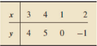
ŷ = -3 + 2x
Expert Solution & Answer
Want to see the full answer?
Check out a sample textbook solution
Students have asked these similar questions
Regression and Predictions. Exercises 13–28 use the same data sets as Exercises 13–28 in Section 10-1. In each case, find the regression equation, letting the first variable be the predictor (x) variable. Find the indicated predicted value by following the prediction procedure summarized in Figure 10-5 on page 493.
Oscars Using the listed actress/actor ages, find the best predicted age of the Best Actor given that the age of the Best Actress is 54 years. Is the result reasonably close to the Best Actor’s (Eddie Redmayne) actual age of 33 years, which happened in 2015, when the Best Actress was Julianne Moore, who was 54 years of age?
Regression and Predictions. Exercises 13–28 use the same data sets as Exercises 13–28 in Section 10-1. In each case, find the regression equation, letting the first variable be the predictor (x) variable. Find the indicated predicted value by following the prediction procedure summarized in Figure 10-5 on page 493.
Internet and Nobel Laureates Find the best predicted Nobel Laureate rate for Japan, which has 79.1 Internet users per 100 people. How does it compare to Japan’s Nobel Laureate rate of 1.5 per 10 million people?
Making Predictions. In Exercises 5–8, let the predictor variable x be the first variable given. Use the given data to find the regression equation and the best predicted value of the response variable. Be sure to follow the prediction procedure summarized in Figure 10-5 on page 493. Use a 0.05 significance level.
Bear Measurements Head widths (in.) and weights (lb) were measured for 20 randomly selected bears (from Data Set 9 “Bear Measurements” in Appendix B). The 20 pairs of measurements yield x = 6.9 in., ȳ = 214.3 lb, r = 0.879, P -value = 0.000, and ŷ = −212 + 61.9x. Find the best predicted value of ŷ (weight) given a bear with a head width of 6.5 in.
Chapter 15 Solutions
Introductory Statistics (10th Edition)
Ch. 15.1 - Suppose that x and y are predictor and response...Ch. 15.1 - Prob. 2ECh. 15.1 - Prob. 3ECh. 15.1 - Prob. 4ECh. 15.1 - Prob. 5ECh. 15.1 - In Exercises 15.315.6, assume that the variables...Ch. 15.1 - The difference between an observed value and a...Ch. 15.1 - Identify two graphs used in a residual analysis to...Ch. 15.1 - Which graph used in a residual analysis provides...Ch. 15.1 - Figure 15.8 shows three residual plots and a...
Ch. 15.1 - Figure 15.9 on the next page shows three residual...Ch. 15.1 - In Exercises 15.1215.21, we repeat the data and...Ch. 15.1 - In Exercises 15.1215.21, we repeat the data and...Ch. 15.1 - Prob. 14ECh. 15.1 - Prob. 15ECh. 15.1 - Prob. 16ECh. 15.1 - Prob. 17ECh. 15.1 - Prob. 18ECh. 15.1 - Prob. 19ECh. 15.1 - Prob. 20ECh. 15.1 - Prob. 21ECh. 15.1 - Prob. 22ECh. 15.1 - Prob. 23ECh. 15.1 - Prob. 24ECh. 15.1 - Prob. 25ECh. 15.1 - In Exercises 15.2215.27, we repeat the information...Ch. 15.1 - Prob. 27ECh. 15.1 - Prob. 28ECh. 15.1 - In Exercises 15.2815.33, a. compute the standard...Ch. 15.1 - Prob. 30ECh. 15.1 - In Exercises 15.2815.33, a. compute the standard...Ch. 15.1 - In Exercises 15.2815.33, a. compute the standard...Ch. 15.1 - In Exercises 15.2815.33, a. compute the standard...Ch. 15.1 - In Exercises 15.3415.43, use the technology of...Ch. 15.1 - In Exercises 15.3415.43, use the technology of...Ch. 15.1 - In Exercises 15.3415.43, use the technology of...Ch. 15.1 - In Exercises 15.3415.43, use the technology of...Ch. 15.1 - Prob. 38ECh. 15.1 - Prob. 39ECh. 15.1 - Prob. 40ECh. 15.1 - Prob. 41ECh. 15.1 - Prob. 42ECh. 15.1 - Prob. 43ECh. 15.2 - Explain why the predictor variable is useless as a...Ch. 15.2 - Prob. 45ECh. 15.2 - Prob. 46ECh. 15.2 - In this section, we used the statistic b1 as a...Ch. 15.2 - In Exercises 15.4815.57, we repeat the information...Ch. 15.2 - Prob. 49ECh. 15.2 - In Exercises 15.4815.57, we repeat the information...Ch. 15.2 - In Exercises 15.4815.57, we repeat the information...Ch. 15.2 - Prob. 52ECh. 15.2 - Prob. 53ECh. 15.2 - Prob. 54ECh. 15.2 - In Exercises 15.4815.57, we repeat the information...Ch. 15.2 - Prob. 56ECh. 15.2 - Prob. 57ECh. 15.2 - Prob. 58ECh. 15.2 - In Exercises 15.5815.63, we repeat the information...Ch. 15.2 - Prob. 60ECh. 15.2 - In Exercises 15.5815.63, we repeat the information...Ch. 15.2 - Prob. 62ECh. 15.2 - In Exercises 15.5815.63, we repeat the information...Ch. 15.2 - Prob. 64ECh. 15.2 - In each of Exercises 15.6415.69, apply Procedure...Ch. 15.2 - In each of Exercises 15.6415.69, apply Procedure...Ch. 15.2 - Prob. 67ECh. 15.2 - Prob. 68ECh. 15.2 - Prob. 69ECh. 15.2 - Prob. 70ECh. 15.2 - In Exercises 15.7015.80, use the technology of...Ch. 15.2 - In Exercises 15.7015.80, use the technology of...Ch. 15.2 - Prob. 73ECh. 15.2 - Prob. 74ECh. 15.2 - Prob. 75ECh. 15.2 - In Exercises 15.7015.80, use the technology of...Ch. 15.2 - Prob. 77ECh. 15.2 - Prob. 78ECh. 15.2 - In Exercises 15.7015.80, use the technology of...Ch. 15.2 - Prob. 80ECh. 15.3 - Without doing any calculations, fill in the blank....Ch. 15.3 - Prob. 82ECh. 15.3 - Prob. 83ECh. 15.3 - Prob. 84ECh. 15.3 - In Exercises 15.8215.91, we repeat the data from...Ch. 15.3 - Prob. 86ECh. 15.3 - Prob. 87ECh. 15.3 - In Exercises 15.8215.91, we repeat the data from...Ch. 15.3 - Prob. 89ECh. 15.3 - Prob. 90ECh. 15.3 - Prob. 91ECh. 15.3 - Prob. 92ECh. 15.3 - In Exercises 15.9215.97, presume that the...Ch. 15.3 - In Exercises 15.9215.97, presume that the...Ch. 15.3 - In Exercises 15.9215.9, presume that the...Ch. 15.3 - Prob. 96ECh. 15.3 - In Exercises 15.9215.97, presume that the...Ch. 15.3 - Prob. 98ECh. 15.3 - In Exercises 15.9815.108, use the technology of...Ch. 15.3 - In Exercises 15.9815.108, use the technology of...Ch. 15.3 - In Exercises 15.9815.108, use the technology of...Ch. 15.3 - In Exercises 15.9815.108, use the technology of...Ch. 15.3 - Prob. 103ECh. 15.3 - Prob. 104ECh. 15.3 - Prob. 105ECh. 15.3 - Prob. 106ECh. 15.3 - In Exercises 15.9815.108, use the technology of...Ch. 15.3 - Prob. 108ECh. 15.3 - Margin of Error in Regression. In Exercises 15.109...Ch. 15.3 - Refer to the confidence interval and prediction...Ch. 15.4 - Identify the statistic used to estimate the...Ch. 15.4 - Prob. 112ECh. 15.4 - Suppose that, for a sample of pairs of...Ch. 15.4 - Prob. 114ECh. 15.4 - Prob. 115ECh. 15.4 - Prob. 116ECh. 15.4 - Prob. 117ECh. 15.4 - Prob. 118ECh. 15.4 - Prob. 119ECh. 15.4 - Prob. 120ECh. 15.4 - Prob. 121ECh. 15.4 - Prob. 122ECh. 15.4 - Prob. 123ECh. 15.4 - Prob. 124ECh. 15.4 - Prob. 125ECh. 15.4 - Prob. 126ECh. 15.4 - Prob. 127ECh. 15.4 - Prob. 128ECh. 15.4 - Prob. 129ECh. 15.4 - Prob. 130ECh. 15.4 - Prob. 131ECh. 15.4 - Prob. 132ECh. 15.4 - Prob. 133ECh. 15.4 - In each of Exercises 15.13415.144, use the...Ch. 15.4 - In each of Exercises 15.13415.144, use the...Ch. 15.4 - Prob. 136ECh. 15.4 - Prob. 137ECh. 15.4 - Prob. 138ECh. 15.4 - Prob. 139ECh. 15.4 - Prob. 140ECh. 15.4 - In each of Exercises 15.13415.144, use the...Ch. 15.4 - Prob. 142ECh. 15.4 - Prob. 143ECh. 15.4 - Prob. 144ECh. 15 - Prob. 1RPCh. 15 - Suppose that x and y are two variables of a...Ch. 15 - What two plots did we use in this chapter to...Ch. 15 - Regarding analysis of residuals, decide in each...Ch. 15 - Suppose that you perform a hypothesis test for the...Ch. 15 - Prob. 6RPCh. 15 - Prob. 7RPCh. 15 - Prob. 8RPCh. 15 - Prob. 9RPCh. 15 - Identify the relationship between two variables...Ch. 15 - Graduation Rates. Graduation ratethe percentage of...Ch. 15 - Prob. 12RPCh. 15 - Prob. 13RPCh. 15 - For Problems 1417, presume that the variables...Ch. 15 - For Problems 1417, presume that the variables...Ch. 15 - For Problems 1417, presume that the variables...Ch. 15 - Prob. 17RPCh. 15 - In Problems 1820, use the technology of your...Ch. 15 - In Problems 1820, use the technology of your...Ch. 15 - In Problems 1820, use the technology of your...Ch. 15 - Recall from Chapter 1 (see page 34) that the Focus...Ch. 15 - At the beginning of this chapter, we presented...
Knowledge Booster


Learn more about
Need a deep-dive on the concept behind this application? Look no further. Learn more about this topic, statistics and related others by exploring similar questions and additional content below.Similar questions
- a) Calculate the sample correlation coefficient r (show all your work).b) Calculate the regression line (you may use technology, but you should write up the details).c) Use the regression line obtain in b. to predict the value of y for x = 0.3 year.d) Use the regression line obtain in b. to predict the value of y for x = 0.8 year.arrow_forwardQ1) Interpret the following regression line y = 10.50 – 0.18xarrow_forwardRegression and Predictions. Exercises 13–28 use the same data sets as Exercises 13–28 in Section 10-1. In each case, find the regression equation, letting the first variable be the predictor (x) variable. Find the indicated predicted value by following the prediction procedure summarized in Figure 10-5 on page 493. Crickets and Temperature Find the best predicted temperature at a time when a cricket chirps 3000 times in 1 minute. What is wrong with this predicted temperature?arrow_forward
- Given the regression line Ý = 2.5X +12, what is the predicted value of self-esteem where X = 5? O 14 O 12.5 O 24.5 22arrow_forwardInterpreting a Computer Display. In Exercises 5–8, we want to consider the correlation between heights of fathers and mothers and the heights of their sons. Refer to the StatCrunch display and answer the given questions or identify the indicated items. The display is based on Data Set 5 “Family Heights” in Appendix B. Height of Son A son will be bom to a father who is 70 in. tall and a mother who is 60 in. tall. Use the multiple regression equation to predict the height of the son. Is the result likely to be a good predicted value? Why or why not?arrow_forwardYou conducted a regression analysis between the number of absences and number of tasks missed by your 5 classmates in Statistics and Probability. It resulted that the regression line is y = 0.65x + 1.18. What is the predicted number of tasks missed of a learner who is always present? O a. The learner has 1 task missed. O b. The learner has less than 2 tasks missed. O c. The learner has more than 2 tasks missed. o d. The learner has no task missed.arrow_forward
- Sam Jones has 2 years of historical sales data for his company. He is applyingfor a business loan and must supply his projections of sales by month for thenext 2 years to the bank. a. Using the data from Table 6–12, provide a regression forecast for timeperiods 25 through 48.b. Does Sam’s sales data show a seasonal pattern?arrow_forwardRegression and Predictions. Exercises 13–28 use the same data sets as Exercises 13–28 in Section 10-1. In each case, find the regression equation, letting the first variable be the predictor (x) variable. Find the indicated predicted value by following the prediction procedure summarized in Figure 10-5 on page 493. Tips Using the bill/tip data, find the best predicted tip amount for a dinner bill of $100. What tipping rule does the regression equation suggest?arrow_forward3. Create two new independent variables: Top 2–5 and Top 6–10. Top 2–5 represents the number of times the driver finished between second and fifth place and Top 6–10 represents the number of times the driver finished between sixth and tenth place. Develop an estimated regression equation that can be used to predict Winnings ($) using Poles, Wins, Top 2–5, and Top 6–10. Test for individual significance and discuss your findings and conclusions. Driver Points Poles Wins Top 5 Top 10 Winnings ($) Tony Stewart 2403 1 5 9 19 6,529,870 Carl Edwards 2403 3 1 19 26 8,485,990 Kevin Harvick 2345 0 4 9 19 6,197,140 Matt Kenseth 2330 3 3 12 20 6,183,580 Brad Keselowski 2319 1 3 10 14 5,087,740 Jimmie Johnson 2304 0 2 14 21 6,296,360 Dale Earnhardt Jr. 2290 1 0 4 12 4,163,690 Jeff Gordon 2287 1 3 13 18 5,912,830 Denny Hamlin 2284 0 1 5 14 5,401,190 Ryan Newman 2284 3 1 9 17 5,303,020 Kurt Busch 2262 3 2 8 16 5,936,470 Kyle Busch 2246 1 4 14 18 6,161,020 Clint Bowyer…arrow_forward
- 3. Regression analysis breaks scores on the DV into... (explain and give equations)arrow_forwardQuestion 3. a) A Biologist is comparing intervals (m seconds) between the matting calls of a certain species of tree frog and the surrounding temperature (t degree Celsius). The following results were obtained: t 8 13 14 15 15 20 25 30 6.5 4.5 4 3 2 1 1. Fit the regression line in the form m = a + bt. 2. Interpret your estimates. 3. Use your regression line interval between matting calls when the surrounding temperature is 10 degrees. (6 marks) estimate the timearrow_forwardInterpreting a Computer Display. In Exercises 5–8, we want to consider the correlation between heights of fathers and mothers and the heights of their sons. Refer to the StatCrunch display and answer the given questions or identify the indicated items. The display is based on Data Set 5 “Family Heights” in Appendix B. Height of Son Identify the multiple regression equation that expresses the height of a son in terms of the height of his father and mother.arrow_forward
arrow_back_ios
SEE MORE QUESTIONS
arrow_forward_ios
Recommended textbooks for you
 MATLAB: An Introduction with ApplicationsStatisticsISBN:9781119256830Author:Amos GilatPublisher:John Wiley & Sons Inc
 Probability and Statistics for Engineering and th...StatisticsISBN:9781305251809Author:Jay L. DevorePublisher:Cengage Learning
 Statistics for The Behavioral Sciences (MindTap C...StatisticsISBN:9781305504912Author:Frederick J Gravetter, Larry B. WallnauPublisher:Cengage Learning
 Elementary Statistics: Picturing the World (7th E...StatisticsISBN:9780134683416Author:Ron Larson, Betsy FarberPublisher:PEARSON
 The Basic Practice of StatisticsStatisticsISBN:9781319042578Author:David S. Moore, William I. Notz, Michael A. FlignerPublisher:W. H. Freeman
 Introduction to the Practice of StatisticsStatisticsISBN:9781319013387Author:David S. Moore, George P. McCabe, Bruce A. CraigPublisher:W. H. Freeman
MATLAB: An Introduction with Applications
Statistics
ISBN:9781119256830
Author:Amos Gilat
Publisher:John Wiley & Sons Inc
Probability and Statistics for Engineering and th...
Statistics
ISBN:9781305251809
Author:Jay L. Devore
Publisher:Cengage Learning
Statistics for The Behavioral Sciences (MindTap C...
Statistics
ISBN:9781305504912
Author:Frederick J Gravetter, Larry B. Wallnau
Publisher:Cengage Learning
Elementary Statistics: Picturing the World (7th E...
Statistics
ISBN:9780134683416
Author:Ron Larson, Betsy Farber
Publisher:PEARSON
The Basic Practice of Statistics
Statistics
ISBN:9781319042578
Author:David S. Moore, William I. Notz, Michael A. Fligner
Publisher:W. H. Freeman
Introduction to the Practice of Statistics
Statistics
ISBN:9781319013387
Author:David S. Moore, George P. McCabe, Bruce A. Craig
Publisher:W. H. Freeman
Correlation Vs Regression: Difference Between them with definition & Comparison Chart; Author: Key Differences;https://www.youtube.com/watch?v=Ou2QGSJVd0U;License: Standard YouTube License, CC-BY
Correlation and Regression: Concepts with Illustrative examples; Author: LEARN & APPLY : Lean and Six Sigma;https://www.youtube.com/watch?v=xTpHD5WLuoA;License: Standard YouTube License, CC-BY