
Introductory Statistics (10th Edition)
10th Edition
ISBN: 9780321989178
Author: Neil A. Weiss
Publisher: PEARSON
expand_more
expand_more
format_list_bulleted
Videos
Textbook Question
Chapter 15.1, Problem 26E
In Exercises 15.22–15.27, we repeat the information from Exercises 14.58–14.63. For each exercise here, discuss what satisfying Assumptions 1–3 for regression inferences by the variables under consideration would mean.
15.26 Crown-Rump Length. In the article “The Human Vomeronasal Organ. Part II: Prenatal Development” (Journal of Anatomy, Vol. 197, Issue 3, pp. 421–136), T. Smith and K. Bhatnagar examined the controversial issue of the human vomeronasal organ, regarding its structure,
Expert Solution & Answer
Want to see the full answer?
Check out a sample textbook solution
Students have asked these similar questions
PLS SHOW COMPLETE SOLUTION. DONT ROUND OFF. USE Z-TABLE.
A)Test the claim, at the a = 0.10 level of significance, that a linear relation exists
between the two variables, for the data below, given that y-1.885x +0.758.
-5 |-3| 4
11 6
y
Step 1) State the null and alternative hypotheses.
Step 2) Determine the critical value for the level of significance, a.
Step 3) Find the test statistic or P-value.
Step 4) Will the researcher reject the null hypothesis or do not the null hypothesis?
Step 5) Write the conclusion.
B) The regression line for the given data is v = -1.885x + 0.758. Determine the
residual of a data point for which x = 2 and y = -4.
SAMSUNG
DII
96
&
Attached to the end of the page is a portion of a printout from a stepwise regression analysis. a) Any of the F statistics on the printout can be computed via the formula:
F = (SSReg( Model A ) – SSReg( Model B ) ) / C
MSResidual( Model A)
Identify what Model A, Model B, and the constant C are in order to obtain the F = 1.33 value for the variable x8 .
b) Based on the printout for Step 6 of the stepwise selection procedure, what will be the next change in the model, in Step 7 of the procedure? (In other words, will a particular term be dropped, or added, or will nothing occur? Assume that the significance level for entry and staying are a = .15.)
Chapter 15 Solutions
Introductory Statistics (10th Edition)
Ch. 15.1 - Suppose that x and y are predictor and response...Ch. 15.1 - Prob. 2ECh. 15.1 - Prob. 3ECh. 15.1 - Prob. 4ECh. 15.1 - Prob. 5ECh. 15.1 - In Exercises 15.315.6, assume that the variables...Ch. 15.1 - The difference between an observed value and a...Ch. 15.1 - Identify two graphs used in a residual analysis to...Ch. 15.1 - Which graph used in a residual analysis provides...Ch. 15.1 - Figure 15.8 shows three residual plots and a...
Ch. 15.1 - Figure 15.9 on the next page shows three residual...Ch. 15.1 - In Exercises 15.1215.21, we repeat the data and...Ch. 15.1 - In Exercises 15.1215.21, we repeat the data and...Ch. 15.1 - Prob. 14ECh. 15.1 - Prob. 15ECh. 15.1 - Prob. 16ECh. 15.1 - Prob. 17ECh. 15.1 - Prob. 18ECh. 15.1 - Prob. 19ECh. 15.1 - Prob. 20ECh. 15.1 - Prob. 21ECh. 15.1 - Prob. 22ECh. 15.1 - Prob. 23ECh. 15.1 - Prob. 24ECh. 15.1 - Prob. 25ECh. 15.1 - In Exercises 15.2215.27, we repeat the information...Ch. 15.1 - Prob. 27ECh. 15.1 - Prob. 28ECh. 15.1 - In Exercises 15.2815.33, a. compute the standard...Ch. 15.1 - Prob. 30ECh. 15.1 - In Exercises 15.2815.33, a. compute the standard...Ch. 15.1 - In Exercises 15.2815.33, a. compute the standard...Ch. 15.1 - In Exercises 15.2815.33, a. compute the standard...Ch. 15.1 - In Exercises 15.3415.43, use the technology of...Ch. 15.1 - In Exercises 15.3415.43, use the technology of...Ch. 15.1 - In Exercises 15.3415.43, use the technology of...Ch. 15.1 - In Exercises 15.3415.43, use the technology of...Ch. 15.1 - Prob. 38ECh. 15.1 - Prob. 39ECh. 15.1 - Prob. 40ECh. 15.1 - Prob. 41ECh. 15.1 - Prob. 42ECh. 15.1 - Prob. 43ECh. 15.2 - Explain why the predictor variable is useless as a...Ch. 15.2 - Prob. 45ECh. 15.2 - Prob. 46ECh. 15.2 - In this section, we used the statistic b1 as a...Ch. 15.2 - In Exercises 15.4815.57, we repeat the information...Ch. 15.2 - Prob. 49ECh. 15.2 - In Exercises 15.4815.57, we repeat the information...Ch. 15.2 - In Exercises 15.4815.57, we repeat the information...Ch. 15.2 - Prob. 52ECh. 15.2 - Prob. 53ECh. 15.2 - Prob. 54ECh. 15.2 - In Exercises 15.4815.57, we repeat the information...Ch. 15.2 - Prob. 56ECh. 15.2 - Prob. 57ECh. 15.2 - Prob. 58ECh. 15.2 - In Exercises 15.5815.63, we repeat the information...Ch. 15.2 - Prob. 60ECh. 15.2 - In Exercises 15.5815.63, we repeat the information...Ch. 15.2 - Prob. 62ECh. 15.2 - In Exercises 15.5815.63, we repeat the information...Ch. 15.2 - Prob. 64ECh. 15.2 - In each of Exercises 15.6415.69, apply Procedure...Ch. 15.2 - In each of Exercises 15.6415.69, apply Procedure...Ch. 15.2 - Prob. 67ECh. 15.2 - Prob. 68ECh. 15.2 - Prob. 69ECh. 15.2 - Prob. 70ECh. 15.2 - In Exercises 15.7015.80, use the technology of...Ch. 15.2 - In Exercises 15.7015.80, use the technology of...Ch. 15.2 - Prob. 73ECh. 15.2 - Prob. 74ECh. 15.2 - Prob. 75ECh. 15.2 - In Exercises 15.7015.80, use the technology of...Ch. 15.2 - Prob. 77ECh. 15.2 - Prob. 78ECh. 15.2 - In Exercises 15.7015.80, use the technology of...Ch. 15.2 - Prob. 80ECh. 15.3 - Without doing any calculations, fill in the blank....Ch. 15.3 - Prob. 82ECh. 15.3 - Prob. 83ECh. 15.3 - Prob. 84ECh. 15.3 - In Exercises 15.8215.91, we repeat the data from...Ch. 15.3 - Prob. 86ECh. 15.3 - Prob. 87ECh. 15.3 - In Exercises 15.8215.91, we repeat the data from...Ch. 15.3 - Prob. 89ECh. 15.3 - Prob. 90ECh. 15.3 - Prob. 91ECh. 15.3 - Prob. 92ECh. 15.3 - In Exercises 15.9215.97, presume that the...Ch. 15.3 - In Exercises 15.9215.97, presume that the...Ch. 15.3 - In Exercises 15.9215.9, presume that the...Ch. 15.3 - Prob. 96ECh. 15.3 - In Exercises 15.9215.97, presume that the...Ch. 15.3 - Prob. 98ECh. 15.3 - In Exercises 15.9815.108, use the technology of...Ch. 15.3 - In Exercises 15.9815.108, use the technology of...Ch. 15.3 - In Exercises 15.9815.108, use the technology of...Ch. 15.3 - In Exercises 15.9815.108, use the technology of...Ch. 15.3 - Prob. 103ECh. 15.3 - Prob. 104ECh. 15.3 - Prob. 105ECh. 15.3 - Prob. 106ECh. 15.3 - In Exercises 15.9815.108, use the technology of...Ch. 15.3 - Prob. 108ECh. 15.3 - Margin of Error in Regression. In Exercises 15.109...Ch. 15.3 - Refer to the confidence interval and prediction...Ch. 15.4 - Identify the statistic used to estimate the...Ch. 15.4 - Prob. 112ECh. 15.4 - Suppose that, for a sample of pairs of...Ch. 15.4 - Prob. 114ECh. 15.4 - Prob. 115ECh. 15.4 - Prob. 116ECh. 15.4 - Prob. 117ECh. 15.4 - Prob. 118ECh. 15.4 - Prob. 119ECh. 15.4 - Prob. 120ECh. 15.4 - Prob. 121ECh. 15.4 - Prob. 122ECh. 15.4 - Prob. 123ECh. 15.4 - Prob. 124ECh. 15.4 - Prob. 125ECh. 15.4 - Prob. 126ECh. 15.4 - Prob. 127ECh. 15.4 - Prob. 128ECh. 15.4 - Prob. 129ECh. 15.4 - Prob. 130ECh. 15.4 - Prob. 131ECh. 15.4 - Prob. 132ECh. 15.4 - Prob. 133ECh. 15.4 - In each of Exercises 15.13415.144, use the...Ch. 15.4 - In each of Exercises 15.13415.144, use the...Ch. 15.4 - Prob. 136ECh. 15.4 - Prob. 137ECh. 15.4 - Prob. 138ECh. 15.4 - Prob. 139ECh. 15.4 - Prob. 140ECh. 15.4 - In each of Exercises 15.13415.144, use the...Ch. 15.4 - Prob. 142ECh. 15.4 - Prob. 143ECh. 15.4 - Prob. 144ECh. 15 - Prob. 1RPCh. 15 - Suppose that x and y are two variables of a...Ch. 15 - What two plots did we use in this chapter to...Ch. 15 - Regarding analysis of residuals, decide in each...Ch. 15 - Suppose that you perform a hypothesis test for the...Ch. 15 - Prob. 6RPCh. 15 - Prob. 7RPCh. 15 - Prob. 8RPCh. 15 - Prob. 9RPCh. 15 - Identify the relationship between two variables...Ch. 15 - Graduation Rates. Graduation ratethe percentage of...Ch. 15 - Prob. 12RPCh. 15 - Prob. 13RPCh. 15 - For Problems 1417, presume that the variables...Ch. 15 - For Problems 1417, presume that the variables...Ch. 15 - For Problems 1417, presume that the variables...Ch. 15 - Prob. 17RPCh. 15 - In Problems 1820, use the technology of your...Ch. 15 - In Problems 1820, use the technology of your...Ch. 15 - In Problems 1820, use the technology of your...Ch. 15 - Recall from Chapter 1 (see page 34) that the Focus...Ch. 15 - At the beginning of this chapter, we presented...
Knowledge Booster


Learn more about
Need a deep-dive on the concept behind this application? Look no further. Learn more about this topic, statistics and related others by exploring similar questions and additional content below.Similar questions
- Please show me your solutions and interpretations. Show the completehypothesis-testing procedure.An article in the ASCE Journal of Energy Engineering (1999, Vol. 125, pp. 59–75) describes a study of the thermal inertia properties of autoclaved aerated concrete used as a building material. Five samples of the material were tested in a structure, and the average interior temperatures (°C) reported were as follows: 23.01, 22.22, 22.04, 22.62, and 22.59. Test that the average interior temperature is equal to 22.5 °C using α = 0.05.arrow_forwardCity Fuel Consumption: Finding the Best Multiple Regression Equation. In Exercises 9–12, refer to the accompanying table, which was obtained using the data from 21 cars listed in Data Set 20 “Car Measurements” in Appendix B. The response (y) variable is CITY (fuel consumption in mi/gal). The predictor (x) variables are WT (weight in pounds), DISP (engine displacement in liters), and HWY (highway fuel consumption in mi /gal). A Honda Civic weighs 2740 lb, it has an engine displacement of 1.8 L, and its highway fuel consumption is 36 mi/gal. What is the best predicted value of the city fuel consumption? Is that predicted value likely to be a good estimate? Is that predicted value likely to be very accurate?arrow_forwardCity Fuel Consumption: Finding the Best Multiple Regression Equation. In Exercises 9–12, refer to the accompanying table, which was obtained using the data from 21 cars listed in Data Set 20 “Car Measurements” in Appendix B. The response (y) variable is CITY (fuel consumption in mi/gal). The predictor (x) variables are WT (weight in pounds), DISP (engine displacement in liters), and HWY (highway fuel consumption in mi /gal). Which regression equation is best for predicting city fuel consumption? Why?arrow_forward
- City Fuel Consumption: Finding the Best Multiple Regression Equation. In Exercises 9–12, refer to the accompanying table, which was obtained using the data from 21 cars listed in Data Set 20 “Car Measurements” in Appendix B. The response (y) variable is CITY (fuel consumption in mi/gal). The predictor (x) variables are WT (weight in pounds), DISP (engine displacement in liters), and HWY (highway fuel consumption in mi /gal). If exactly two predictor (x) variables are to be used to predict the city fuel consumption, which two variables should be chosen? Why?arrow_forwardYou have estimated a multiple regression model with 6 explanatory variables and an intercept from a sample with 46 observations. What is the critical value of the test statistic (tc) if you want to perform a test for the significance of a single right-hand side (explanatory) variable at α = 0.05? a.) 2.023 b.) 2.708 c.) 2.423 d.) 2.704arrow_forwardWhich non-parametric test for ordinal data is the best to use in the given scenario? In a study by Zuckerman and Heneghan, hemodynamic stresses were measured on subjects undergoing laparoscopic cholecystectomy. An outcome variable of interest was the ventricular end-diastolic volume (LVEDV) measured in mm. A portion of the data appears in the following table. Baseline refers to a measurement taken 5 minutes after induction of anesthesia, and the term '5 minutes' refers to a measurement taken 5 minutes after baseline. Can we conclude that, on the basis of these data, among subjects undergoing laparoscopic cholecystectomy, the average LVEDV levels change? Let a =.01. LVEDV (ml) Subject Baseline 5 minutes 1 51.7 49.3 2 79.0 72.0 3 78.7 67.0 4 80.3 70.4 5 72.0 65.9 6 85.0 84.8 7 79.0 77.7 8 71.3 74.0 9 54.3 58.0 10 58.8 65.0 a. Mood Median Test b. Sign Test c. Wilcoxon Rank Sum Test d. Wilcoxon Matched-Pair Signed-Ranks Test e. Spearman and Kendall Correlation…arrow_forward
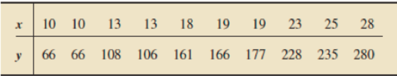
- Q.2 Since outbreak of COVID-19 pandemic insurance companies started spending on Advertisement of Corona Kavach policy to enhance the revenue due to rising number of cases in India. The data below explains the advertising expenditure and revenue of seven companies. a) Is there any association between advertising expenditure and revenue earned ? b) Use the data to develop a regression line to predict the amount of advertising by revenues? c) What is your interpretation from the calculations in part a and b respectively? Name of company Advertising (in Rs.) 1073 Revenues (in Rs.) Birla Sunlife 408.2 Bharti Axa 4898 79.7 Religare Health care Мax Bupa Reliance health care HDFC ergo United Insurance 3345 123.0 3296 104.6 2822 | 2577 |829 107.8 118.3 114.6arrow_forwardApply the predictive control law to a fifth-order process:Y(s)/(s)=1/(5s+1)⁵.Evaluate the effect of tuning paramete rJ on the set-pointresponses for values of J=3, 4, 6, and 8 and Δt=5 min.arrow_forwardSuppose you fit the first-order model y = Po + B, x, + B2x2 + B3X3 + B,x4 + B5X5 + ɛ to n=28 data points and obtain SSE = 0.33 and R = 0.94. Complete parts a and b. a. Do the values of SSE and R suggest that the model provides a good fit to the data? Explain. A. Yes. Since R = 0.94 is close to 1, this indicates the model provides a good fit. Also, SSE = 0.33 is fairly small, which indicates the model provides a good fit. B. There is not enough information to decide. No. Since R = 0.94 is close to 1, this indicates the model does not provide a good fit. Also, SSE = 0.33 is fairly small, which indicates the model does not provide a good fit. b. Is the model of any use in predicting Test the null hypothesis Ho: B, = B2 = ... = B5 = 0 against the alternative hypothesis: At least of the %3D parameters B1, B2, B5 is nonzero. Use a = 0.05. The test statistic is (Round to two decimal places as needed.)arrow_forward
- 2arrow_forwardThe data from the table below gives a regression that is a) reliable. b) unreliable. c) unable to determine the reliability.arrow_forwardAs the population ages, there is increasing concern about accident-related injuries to the elderly. An article reported on an experiment in which the maximum lean angle—the farthest a subject is able to lean and still recover in one step—was determined for both a sample of younger females (21–29 years) and a sample of older females (67–81 years). The following observations are consistent with summary data given in the article: YF: 28, 34, 32, 27, 28, 32, 31, 35, 32, 28 OF: 19, 14, 21, 13, 12 Does the data suggest that true average maximum lean angle for older females (OF) is more than 10 degrees smaller than it is for younger females (YF)? State and test the relevant hypotheses at significance level 0.10. (Use ?1 for younger females and ?2 for older females.) H0: ?1 − ?2 = 10Ha: ?1 − ?2 > 10H0: ?1 − ?2 = 10Ha: ?1 − ?2 < 10 H0: ?1 − ?2 = 0Ha: ?1 − ?2 > 0H0: ?1 − ?2 = 0Ha: ?1 − ?2 < 0 Calculate the test statistic and determine the P-value. (Round your test…arrow_forward
arrow_back_ios
SEE MORE QUESTIONS
arrow_forward_ios
Recommended textbooks for you
 Glencoe Algebra 1, Student Edition, 9780079039897...AlgebraISBN:9780079039897Author:CarterPublisher:McGraw Hill
Glencoe Algebra 1, Student Edition, 9780079039897...
Algebra
ISBN:9780079039897
Author:Carter
Publisher:McGraw Hill
Hypothesis Testing using Confidence Interval Approach; Author: BUM2413 Applied Statistics UMP;https://www.youtube.com/watch?v=Hq1l3e9pLyY;License: Standard YouTube License, CC-BY
Hypothesis Testing - Difference of Two Means - Student's -Distribution & Normal Distribution; Author: The Organic Chemistry Tutor;https://www.youtube.com/watch?v=UcZwyzwWU7o;License: Standard Youtube License