Concept explainers
Videos
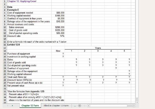
The Excel worksheet form that appears below is to be used to recreate Example E and Exhibit 12-8. Download the workbook containing this form from Connect, where you will also receive instructions about how to use this worksheet form.

 You should proceed to the requirements below only after completing your worksheet. Note that you may get a slightly different
Required:
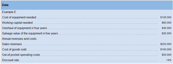
2. The company is considering another project involving the purchase of new equipment. Change the data area of your worksheet to match the following:
a. What is the net present value of the project?
b. Experiment with changing the discount rate in one percent increments (e.g.. 13%. 12%. 15%. etc.). At what interest rate does the net present value turn from negative to positive?
c. The
d. Reset the discount rate to 14%. Suppose the salvage value is uncertain. How large would the salvage value have to be to result in a positive net present value?
1
Net present value NPV is calculated by deducting present value of all the cash inflows from a particular project from the present value of initial cash outflow. NPV helps in identifying the profitability of a project or an investment.
To calculate: The amount of net present value (NPV) for the given project.
Answer to Problem 2AE
NPV is calculated as -$17.340.
Explanation of Solution
Calculation of NPV will be done as follows:
| Particulars | Year 0 ($) | Year 1 ($) | Year 2 ($) | Year 3 ($) | Year 4 ($) | Year 5($) |
| Cost of equipment | -120,000 | |||||
| Working capital needed | -80,000 | |||||
| Sales revenue | 255,000 | 255,000 | 255,000 | 255,000 | 255,000 | |
| Cost of goods sold | -160,000 | -160,000 | -160,000 | -160,000 | -160,000 | |
| Out of pocket operating cost | -50,000 | -50,000 | -50,000 | -50,000 | -50,000 | |
| Working capital released | 80,000 | |||||
| Overhaul cost | -40,000 | |||||
| Salvage value | 20,000 | |||||
| Net cash flow | -200,000 | 45,000 | 45,000 | 45,000 | 5,000 | 145,000 |
| Discount rate (14%) | 1 | 0.877 | 0.769 | 0.675 | 0.592 | 0.519 |
| Present value | -200,000 | 39,465 | 34,605 | 30,375 | 2,960 | 75,255 |
| Net present value (NPV) | -17,340 |
Therefore, NPV is -$17,340.
2
Net present value NPV is calculated by deducting present value of all the cash inflows from a particular project from the present value of initial cash outflow. NPV helps in identifying the profitability of a project or an investment.
The discount rate at which NPV will be positive.
Answer to Problem 2AE
At 10% discount rate NPV will be positive ($5,330).
Explanation of Solution
At 15% discount rate, NPV will be:
| Particulars | Year 0 ($) | Year 1 ($) | Year 2 ($) | Year 3 ($) | Year 4 ($) | Year 5($) |
| Net cash flow | -200,000 | 45,000 | 45,000 | 45,000 | 5,000 | 145,000 |
| Discount rate (15%) | 1 | 0.867 | 0.756 | 0.657 | 0.572 | 0.497 |
| Present value | -200,000 | 39,015 | 34,020 | 29,565 | 2,860 | 72,065 |
| Net present value (NPV) | -22,475 |
At 13% discount rate, NPV will be:
| Particulars | Year 0 ($) | Year 1 ($) | Year 2 ($) | Year 3 ($) | Year 4 ($) | Year 5($) |
| Net cash flow | -200,000 | 45,000 | 45,000 | 45,000 | 5,000 | 145,000 |
| Discount rate (13%) | 1 | 0.885 | 0.783 | 0.693 | 0.613 | 0.543 |
| Present value | -200,000 | 39,825 | 35,235 | 31,185 | 3,065 | 78,735 |
| Net present value (NPV) | -11,955 |
At 12% discount rate, NPV will be:
| Particulars | Year 0 ($) | Year 1 ($) | Year 2 ($) | Year 3 ($) | Year 4 ($) | Year 5($) |
| Net cash flow | -200,000 | 45,000 | 45,000 | 45,000 | 5,000 | 145,000 |
| Discount rate (12%) | 1 | 0.893 | 0.797 | 0.711 | 0.635 | 0.567 |
| Present value | -200,000 | 40,185 | 35,865 | 31,995 | 3,175 | 82,215 |
| Net present value (NPV) | -6,565 |
At 11% discount rate, NPV will be:
| Particulars | Year 0 ($) | Year 1 ($) | Year 2 ($) | Year 3 ($) | Year 4 ($) | Year 5 ($) |
| Net cash flow | -200,000 | 45,000 | 45,000 | 45,000 | 5,000 | 145,000 |
| Discount rate (11%) | 1 | 0.901 | 0.812 | 0.731 | 0.658 | 0.593 |
| Present value | -200,000 | 40,545 | 36,540 | 32,895 | 3,290 | 85,985 |
| Net present value (NPV) | -745 |
At 10% discount rate, NPV will be:
| Particulars | Year 0 ($) | Year 1 ($) | Year 2 ($) | Year 3 ($) | Year 4 ($) | Year 5($) |
| Net cash flow | -200,000 | 45,000 | 45,000 | 45,000 | 5,000 | 145,000 |
| Discount rate (10%) | 1 | 0.909 | 0.826 | 0.751 | 0.683 | 0.621 |
| Present value | -200,000 | 40,905 | 37,170 | 33,795 | 3,415 | 90,045 |
| Net present value (NPV) | 5,330 |
Therefore, NPV will be positive at 10% discount rate.
3
Internal rate of return The interest rate at which NPV of cash flows from an investment is zero is IRR. It helps in identifying if the investment is profitable or not.
IRR is between what two discounting rates.
Answer to Problem 2AE
IRR is 10.884% which is between 10% and 11%.
Explanation of Solution
IRR will be calculated as follows:
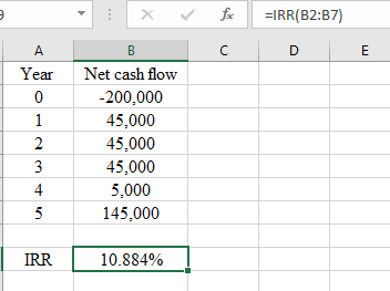
IRR is 10.884% which means that IRR is between 10% and 11%.
Also, IRR is the interest rate at which NPV is zero. At 10%, NPV is $5,330 (calculated in sub part 1) and at 11%, NPV is -745 (Calculated in sub part 1). This also shows that NPV will be zero at some discount rate between 10% and 11%.
4
Salvage value It represents the amount that a company receives by selling an asset at the end of its useful life. It is considered as a cash inflow.
To calculate: The increase in salvage value that will make the NPV positive at 14% discount rate.
Answer to Problem 2AE
Increase in salvage value is $29,560 and total salvage value is $49,560.
Explanation of Solution
| Particulars | Year 0 ($) | Year 1 ($) | Year 2 ($) | Year 3 ($) | Year 4 ($) | Year 5($) |
| Net cash flow | -200,000 | 45,000 | 45,000 | 45,000 | 5,000 | 145,000 |
| Discount rate (14%) | 1 | 0.877 | 0.769 | 0.675 | 0.592 | 0.519 |
| Present value | -200,000 | 39,465 | 34,605 | 30,375 | 2,960 | 75,255 |
| Net present value (NPV) | -17,340 |
At 14%, total cash outflow is -$200,000, present value of total cash inflows is 182,660 and NPV is negative. NPV will be positive if present value of cash flows will increase by $17,500. Therefore, in year 5 present value of salvage value will increase by $17,500. At year 0, total salvage value will be:
NPV will be positive if total salvage value will be $49,560.
Want to see more full solutions like this?
Chapter 12 Solutions
Introduction To Managerial Accounting


- JPL, Inc. has provided its sales and expense data for the most recent period. The Controller has asked you prepare a spreadsheet that shows the related CVP Analysis computations. Use the information included in the Excel Simulation and the Excel functions described below to complete the task.arrow_forwardAnswer the following questions using the Answer Report and the Sensitivity Report on thefollowing page. Support your answers with explanations and the work showed.Your run a company that produces three electrical products – clocks, radios, and toasters. You are asked to figure out how many of each of these things should be produced, and the computer solution (answer report and sensitivity report generated in Microsoft Excel) is given on the next page. 1.) How many of each of the electronic appliances should you make? (Make sure your answer makes sense.)2.) How much will you end up profiting?3.) Which of the constraints are binding? What does the slack for each non-binding constraint represent?arrow_forwardI really need help with this item below. I have tried a few different ways to do this problem, but the top box keeps coming back as incorrect. I know that the amounts are correct, but the first box is wrong for some reason. Please read the feedback boxes and include the appropriate formulas and cell references for this item. This is done through Excel. PLEASE HELP!!!!!! Note that the pictures are the same exact problem, but I used two separate formulas to try and solve this problem.arrow_forward
- Required information (The Excel worksheet form that appears below is to be used to recreate part of the example relating to Turbo Crafters that appears earlier in the chapter.) Download the Applying Excel form and enter formulas in all cells that contain question marks. For example, in cell B13 enter the formula "= B5". After entering formulas in all of the cells that contained question marks, verify that the dollar amounts match the example in the text. Check your worksheet by changing the estimated total amount of the allocation base in the Data area to 50,000 machine-hours, keeping all of the other data the same as in the original example. If your worksheet is operating properly, the predetermined overhead rate should now be $6.00 per machine-hour. If you do not get this answer, find the errors in your worksheet and correct them. Save your completed Applying Excel form to your computer and then upload it here by clicking "Browse." Next, click "Save." You will use this…arrow_forwardFor this problem, there are 10 future value and present value exercises to be solved. Review the printout of the worksheet file COMPOUND that follows these requirements. This file also contains a second sheet called the Answer Sheet. Note that the worksheet is divided into four sections. You have to decide which section is appropriate for each exercise. Open the file COMPOUND from the website for this book at cengagebrain.com. To enter the four formulas in the appropriate cells, use the FV and PV functions for the annuities (see Appendix A in Excel Quick for a discussion of them). Unfortunately Excel does not provide functions for the future value of an amount nor the present value of an amount. Enter the following formulas for FORMULA1 and FORMULA2: FORMULA1: =B6*((1+B8)^B7) FORMULA2: =E6/((1+E8)^AE7) For the annuity calculations (FV and PV), it is important that you enter a value (or cell reference) for type to indicate the timing of the first payment. If the first payment is made…arrow_forwardThe comparative financial statements of Global Technology are as follows: Open the file RATIOA from the website for this book at cengagebrain.com. Enter the formulas in the appropriate cells. Enter your name in cell A1. Save the completed model as RATIOA2. Print the worksheet when done. Also print your formulas. Check figure: Acid test (quick) ratio (cell C58), .82.arrow_forward
- Below you will see three sets of inputs. After inputting all of your formulas, you should be able to use any of these sets of data and have the answers automatically update within excel. Please choose one of the data sets below and input all of the necessary formulas to find the answers. Once you are done, choose a different data set, enter it into your spreadsheet, and check the updated answers to ensure that everything is flowing through the formulas appropriately. A check answer for each one has been provided. Data set #1 Data Section: Actual and Budgeted Unit Sales: April 1,500 May 1,000 June 1,600 July 1,400 August 1,500 September 1,200 Balance Sheet, May 31, 19X5 Cash $8,000 Accounts Receivable 107,800 Merchandise Inventory 52,800 Fixed Assets (net) 130,000 Total assets $298,600 Accounts Payable (merchandise) $74,800 Owner's equity 223,800 Total liabilities & equity $298,600 Average selling price $98 Average purchase cost per unit $55 Desired ending inventory (% of next…arrow_forwardPlease include the excel formulas too! If someone can help me I will give a thumbs up! Please help me with the last two sections that are not filled out yet. Thanks! :)arrow_forwardPlease help fill out the attached excel example to answer instructions of problem 13-13! Instead of just whoing the correct answers, can you please include the formula you used to get the answers so I can learn how to do the work! Thank you!arrow_forward
- Please do it on EXCEL ONLY. I just want Modified IRR in all three approaches: The discounting approach, the reinvestment approach, and the combination approach. Please post two screenshots, one showing the answers, another showing the formulas in excel.arrow_forwardI need help to do questions 8, 9, and 11 for the Excel Worksheet. Also, please make sure that you provide the steps carefully and get to understand the work as possible. Those questions that I will provide you would be from Microsoft Word.arrow_forwardUsing Excel, create a table that shows the relationship between the interestearned and the amount deposited, as shown. we will first create the dollar amount column and the interest row, as shown . Next we will type into cell B3 the formula = $A3*B$2. We can now use the Fill command to copy the formula in other cells, resulting in the table as shown. Note that the dollar sign before A3 means column A is to remain unchanged in the calculations when the formula is copied into other cells. Also note that the dollar sign before 2 means that row 2 is to remain unchanged in calculations when the Fill command is used.arrow_forward
 Excel Applications for Accounting PrinciplesAccountingISBN:9781111581565Author:Gaylord N. SmithPublisher:Cengage Learning