
Mathematical Statistics with Applications
7th Edition
ISBN: 9780495110811
Author: Dennis Wackerly, William Mendenhall, Richard L. Scheaffer
Publisher: Cengage Learning
expand_more
expand_more
format_list_bulleted
Concept explainers
Videos
Textbook Question
Chapter 11, Problem 96SE
A study was conducted to determine whether a linear relationship exists between the breaking strength y of wooden beams and the specific gravity x of the wood. Ten randomly selected beams of the same cross-sectional dimensions were stressed until they broke. The breaking strengths and the density of the wood are shown in the accompanying table for each of the ten beams.
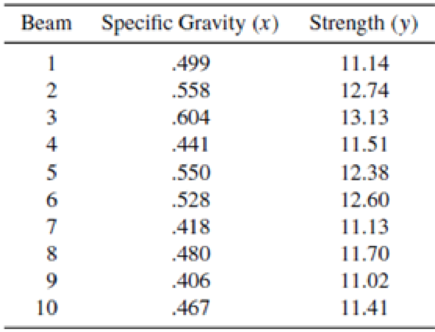
- a Fit the model Y = β0 + β1 x + ε.
- b Test H0: β1 = 0 against the alternative hypothesis, Ha: β1 ≠ 0.
- c Estimate the
mean strength for beams with specific gravity .590, using a 90% confidence interval.
Expert Solution & Answer

Trending nowThis is a popular solution!

Students have asked these similar questions
Arm circumferences (cm) and heights (cm) are measured from randomly selected adult females. The 146pairs of measurements yield x=34.69cm,
y=163.25cm, r=0.075, P-value=0.368, and y=157+0.1826x. Find the best predicted value of y (height) given an adult female with an arm circumference of 40.0cm. Let the predictor variable x be arm circumference and the response variable y be height. Use a 0.05 significance level.
The best predicted value is ____cm.
An experiment to compare the tension bond strength of polymer latex modified mortar (Portland cement mortar to which polymer latex emulsions have been added during mixing) to that of unmodified mortar resulted in x = 18.19 kgf/cm? for the
modified mortar (m = 42) and y = 16.85 kgf/cm? for the unmodified mortar (n = 30). Let u, and u, be the true average tension bond strengths for the modified and unmodified mortars, respectively. Assume that the bond strength distributions are both
normal.
Assuming that o, = 1.6 and o, = 1.3, test Hn: 4, - H, = 0 versus H: u, - u, > 0 at level 0.01.
Calculate the test statistic and determine the P-value. (Round your test statistic to two decimal places and your P-value to four decimal places.)
P-value =
Compute the probability of a type II error for the test of part (a) when 4 - Hz = 1. (Round your answer to four decimal places.)
Suppose the investigator decided to use a level 0.05 test and vwished B = 0.10 when u, - uz = 1. If m = 42, what value of n…
Suppose you fit the first-order model y = Po + B, x, + B2x2 + B3X3 + B,x4 + B5X5 + ɛ to n=28 data points and obtain SSE = 0.33 and R = 0.94. Complete
parts a and b.
a. Do the values of SSE and R suggest that the model provides a good fit to the data? Explain.
A.
Yes. Since R = 0.94 is close to 1, this indicates the model provides a good fit. Also, SSE = 0.33 is fairly small, which indicates the model
provides a good fit.
B. There is not enough information to decide.
No. Since R = 0.94 is close to 1, this indicates the model does not provide a good fit. Also, SSE = 0.33 is fairly small, which indicates the
model does not provide a good fit.
b. Is the model of any use in predicting
Test the null hypothesis Ho: B, = B2 = ... = B5 = 0 against the alternative hypothesis: At least
of the
%3D
parameters B1, B2,
B5 is nonzero. Use a = 0.05.
The test statistic is
(Round to two decimal places as needed.)
Chapter 11 Solutions
Mathematical Statistics with Applications
Ch. 11.3 - If 0 and 1 are the least-squares estimates for the...Ch. 11.3 - Prob. 2ECh. 11.3 - Fit a straight line to the five data points in the...Ch. 11.3 - Auditors are often required to compare the audited...Ch. 11.3 - Prob. 5ECh. 11.3 - Applet Exercise Refer to Exercises 11.2 and 11.5....Ch. 11.3 - Prob. 7ECh. 11.3 - Laboratory experiments designed to measure LC50...Ch. 11.3 - Prob. 9ECh. 11.3 - Suppose that we have postulated the model...
Ch. 11.3 - Some data obtained by C.E. Marcellari on the...Ch. 11.3 - Processors usually preserve cucumbers by...Ch. 11.3 - J. H. Matis and T. E. Wehrly report the following...Ch. 11.4 - a Derive the following identity:...Ch. 11.4 - An experiment was conducted to observe the effect...Ch. 11.4 - Prob. 17ECh. 11.4 - Prob. 18ECh. 11.4 - A study was conducted to determine the effects of...Ch. 11.4 - Suppose that Y1, Y2,,Yn are independent normal...Ch. 11.4 - Under the assumptions of Exercise 11.20, find...Ch. 11.4 - Prob. 22ECh. 11.5 - Use the properties of the least-squares estimators...Ch. 11.5 - Do the data in Exercise 11.19 present sufficient...Ch. 11.5 - Use the properties of the least-squares estimators...Ch. 11.5 - Let Y1, Y2, . . . , Yn be as given in Exercise...Ch. 11.5 - Prob. 30ECh. 11.5 - Using a chemical procedure called differential...Ch. 11.5 - Prob. 32ECh. 11.5 - Prob. 33ECh. 11.5 - Prob. 34ECh. 11.6 - For the simple linear regression model Y = 0 + 1x...Ch. 11.6 - Prob. 36ECh. 11.6 - Using the model fit to the data of Exercise 11.8,...Ch. 11.6 - Refer to Exercise 11.3. Find a 90% confidence...Ch. 11.6 - Refer to Exercise 11.16. Find a 95% confidence...Ch. 11.6 - Refer to Exercise 11.14. Find a 90% confidence...Ch. 11.6 - Prob. 41ECh. 11.7 - Suppose that the model Y=0+1+ is fit to the n data...Ch. 11.7 - Prob. 43ECh. 11.7 - Prob. 44ECh. 11.7 - Prob. 45ECh. 11.7 - Refer to Exercise 11.16. Find a 95% prediction...Ch. 11.7 - Refer to Exercise 11.14. Find a 95% prediction...Ch. 11.8 - The accompanying table gives the peak power load...Ch. 11.8 - Prob. 49ECh. 11.8 - Prob. 50ECh. 11.8 - Prob. 51ECh. 11.8 - Prob. 52ECh. 11.8 - Prob. 54ECh. 11.8 - Prob. 55ECh. 11.8 - Prob. 57ECh. 11.8 - Prob. 58ECh. 11.8 - Prob. 59ECh. 11.8 - Prob. 60ECh. 11.9 - Refer to Example 11.10. Find a 90% prediction...Ch. 11.9 - Prob. 62ECh. 11.9 - Prob. 63ECh. 11.9 - Prob. 64ECh. 11.9 - Prob. 65ECh. 11.10 - Refer to Exercise 11.3. Fit the model suggested...Ch. 11.10 - Prob. 67ECh. 11.10 - Fit the quadratic model Y=0+1x+2x2+ to the data...Ch. 11.10 - The manufacturer of Lexus automobiles has steadily...Ch. 11.10 - a Calculate SSE and S2 for Exercise 11.4. Use the...Ch. 11.12 - Consider the general linear model...Ch. 11.12 - Prob. 72ECh. 11.12 - Prob. 73ECh. 11.12 - An experiment was conducted to investigate the...Ch. 11.12 - Prob. 75ECh. 11.12 - The results that follow were obtained from an...Ch. 11.13 - Prob. 77ECh. 11.13 - Prob. 78ECh. 11.13 - Prob. 79ECh. 11.14 - Prob. 80ECh. 11.14 - Prob. 81ECh. 11.14 - Prob. 82ECh. 11.14 - Prob. 83ECh. 11.14 - Prob. 84ECh. 11.14 - Prob. 85ECh. 11.14 - Prob. 86ECh. 11.14 - Prob. 87ECh. 11.14 - Prob. 88ECh. 11.14 - Refer to the three models given in Exercise 11.88....Ch. 11.14 - Prob. 90ECh. 11.14 - Prob. 91ECh. 11.14 - Prob. 92ECh. 11.14 - Prob. 93ECh. 11.14 - Prob. 94ECh. 11 - At temperatures approaching absolute zero (273C),...Ch. 11 - A study was conducted to determine whether a...Ch. 11 - Prob. 97SECh. 11 - Prob. 98SECh. 11 - Prob. 99SECh. 11 - Prob. 100SECh. 11 - Prob. 102SECh. 11 - Prob. 103SECh. 11 - An experiment was conducted to determine the...Ch. 11 - Prob. 105SECh. 11 - Prob. 106SECh. 11 - Prob. 107SE
Knowledge Booster


Learn more about
Need a deep-dive on the concept behind this application? Look no further. Learn more about this topic, statistics and related others by exploring similar questions and additional content below.Similar questions
- An experiment to compare the tension bond strength of polymer latex modified mortar (Portland cement mortar to which polymer latex emulsions have been added during mixing) to that of unmodified mortar resulted in x = 18.13 kgf/cm? for the modified mortar (m = 42) and y = 16.85 kgf/cm2 for the unmodified mortar (n = 32). Let u, and u, be the true average tension bond strengths for the modified and unmodified mortars, respectively. Assume that the bond strength distributions are both normal. (a) Assuming that o, = 1.6 and o, = 1.3, test Ho: 4, - H, = 0 versus H: u, - µ, > 0 at level 0.01. Calculate the test statistic and determine the P-value. (Round your test statistic to two decimal places and your p-value to four decimal places.) z = 3.80 P-value = 0.0001 State the conclusion in the problem context. O Fail to reject H,. The data suggests that the difference in average tension bond strengths exceeds 0. O Fail to reject Ho: The data does not suggest that the difference in average…arrow_forwardAn experiment to compare the tension bond strength of polymer latex modified mortar (Portland cement mortar to which polymer latex emulsións have been added during mixing) to that of unmodified mortar resulted in x = 18.11 kgf/cm2 for the modified mortar (m = 42) and y = 16.88 kgf/cm2 for the unmodified mortar (n = 31). Let ₁ and ₂ be the true average tension bond strengths for the modified and unmodified mortars, respectively. Assume that the bond strength distributions are both normal. (a) Assuming that o₁ = 1.6 and ₂ = 1.3, test Ho: ₁ - ₂ = 0 versus H₂: H₁ - H₂> 0 at level 0.01. Calculate the test statistic and determine the P-value. (Round your test statistic to two decimal places and your P-value to four decimal places.) Z = P-value = State the conclusion in the problem context. O Fail to reject Ho. The data suggests that the difference in average tension bond strengths exceeds 0. Fail to reject Ho. The data does not suggest that the difference in average tension bond strengths…arrow_forwardArm circumferences (cm) and heights (cm) are measured from randomly selected adult females. The 143 pairs of measurements yield x = 32.40 cm, y = 160.39 cm, r=0.072, P-value = 0.393, and y = 157 + 0.1075x. Find the best predicted value of y (height) given an adult female with an arm circumference of 34.0 cm. Let the predictor variable x be arm circumference and the response variable y be height. Use a 0.05 significance level. %3D The best predicted value is cm. (Round to two decimal places as needed.) Enter your answer in the answer box. MacBook Pro 888 esc %24 % & 4. 9- E T. Y. H. K %#3arrow_forward
- Suppose that the weight of a type of organism is governed by a power law relationship with its length from snout to tail and the thickness of its central vertebrae W = cLpVq. One specimen weighed 37 kg with a length of 1.6 m and vertebral thickness 1 cm. A second specimen weighed 45 kg with a length of 1.6 m and vertebral thickness 1.3 cm. A third specimen weighed 56 kg with a length of 3.1 m and vertebral thickness 1.2 cm. Write an equation with the correct coefficient and parameters values.arrow_forwardArm circumferences (cm) and heights (cm) are measured from randomly selected adult females. The 148 pairs of measurements yield x= 32.00 cm, y = 162.25 cm, r= 0.044, P-value = 0.596, and y = 159 +0.1111x. Find the best predicted value of y (height) given an adult female with an arm circumference of 32.0 cm. Let the predictor variable x be arm circumference and the response variable y be height. Use a 0.05 significance level. The best predicted value is cm. (Round to two decimal places as needed.)arrow_forwardSolve An article in the ASCE Journal of Energy Engineering (1999, Vol. 125, pp.59-75) describes a study of the thermal inertia properties of autoclaved aerated concrete used as a building material. Five samples of the material were tested in a structure, and the average interior temperatures (°C) reported were as follows: 23.01, 22.22, 22.04, 22.62, and 22.59. Test that the average interior temperature is equal to 22.5°C using alpha (a) = 0.05. 1.)This problem is a test on what population parameter? a.Variance/ Standard Deviation b.Mean c.Population Proportion d.None of the above 2.)What is the null and alternative 3 points hypothesis? a.Ho / (theta = 22.5) , Ha: (0 # 22.5) b.Ho / (theta > 22.5) , Ha: (0 # 22.5) c.Ho / (theta < 22.5) , Ha: (theta >= 22.5) d.None of the above 3.)What are the Significance level 3 points and type of test? alpha = 0.05 two-tailed alpha = 0.95 two-tailed alpha = 0.95 one-tailed None of the above 4.)What standardized test statistic will…arrow_forward
- 6. A study was conducted to determine whether a linear relationship exists between the breaking strength y of wooden beams and the specific gravity x of the wood. Ten randomly selected beams of the same cross-sectional dimensions were stressed until they broke. The breaking strengths and density of the wood for each of the ten beams are shown in the following table. Beam Specific Gravity (x) Strength (y) .499 11.14 .558 12.74 .604 13.13 I1.51 12.38 12.60 .441 550 .528 7 418 11.13 480 406 8 11.70 9 11.02 10 .467 11.41 (a) Estimate the linear regression line. (b) Test H.: B = 0 against the alternative hypothesis H,: B, > 0.arrow_forwardHeights (cm) and weights (kg) are measured for 100 randomly selected adult males, and range from heights of 132 to 194 cm and weights of 38 to 150 kg. Let the predictor variable x be the first variable given. The 100 paired measurements yield x 167.75 cm, y=81.58 kg, r0.318, P.value = 0.001, and y-109 1.14x. Find the best predicted value of y (weight) given an adult male who is 184 cm tal, Use a 0.05 significance level. The best predicted value of y for an adult male who is 184 cm tall is kg. (Round to two decimal places as needed.)arrow_forwardThe sale of eggs that are contaminated with Salmonella can cause food poisoning among consumers. A large egg producer takes an SRS of 200 eggs from all the eggs shipped in one day. The laboratory reports that 11 of these eggs had Salmonella contamination. Unbeknownst to the producer, 0.2% of all eggs shipped had Salmonella. What is the best description of the values, 11 and 0.2%, in this situation? O 11 is a parameter and 0.2% is a statistic. O 0.2% is a parameter and 11 is a statistic. O Both 0.2% and 11 are parameters. Both 0.2% and 11 are statistics.arrow_forward
- The spotted lanternfly, Lycorma delicatula, is an invasive species to the United States that has the potential to do significant agricultural damage. An ecologist is studying the relationship between the size of the female spotted lanternflies and the number of eggs they produce. The data are summarized below. Length of insect: AVG = 1 inch, SD = 0.15 inchNumber of eggs: AVG = 40 eggs, SD = 5 eggsr = 0.2 Using regression, we can say that the average number of eggs produced by female spotted lanternflies who are 1.1 inch long is closest to... Group of answer choices 42 39 40 41arrow_forwardA soft drink manufacturer wants to determine the proportion of its soda cans that meet quality standards. A quality control engineer randomly selects 2000 cans off the assembly line and finds that 99.7% (1994 of the 2000) meet quality standards. Step 2 of 4: What is the parameter of interest?arrow_forwardArm circumferences (cm) and heights (cm) are measured from randomly selected adult females. The 142 pairs of measurements yield x=32.14cm, y=163.36cm, r=.084, P value=.32 and y=160+.111x. Find the best predicted value of y (height) given an adult female with an arm circumference of 40cm. Let the predictor variable x be arm circumference and the response variable y be height. Use a .05 significance level.arrow_forward
arrow_back_ios
SEE MORE QUESTIONS
arrow_forward_ios
Recommended textbooks for you
 Calculus For The Life SciencesCalculusISBN:9780321964038Author:GREENWELL, Raymond N., RITCHEY, Nathan P., Lial, Margaret L.Publisher:Pearson Addison Wesley,
 Algebra & Trigonometry with Analytic GeometryAlgebraISBN:9781133382119Author:SwokowskiPublisher:Cengage
Calculus For The Life Sciences
Calculus
ISBN:9780321964038
Author:GREENWELL, Raymond N., RITCHEY, Nathan P., Lial, Margaret L.
Publisher:Pearson Addison Wesley,
Algebra & Trigonometry with Analytic Geometry
Algebra
ISBN:9781133382119
Author:Swokowski
Publisher:Cengage
Statistics 4.1 Point Estimators; Author: Dr. Jack L. Jackson II;https://www.youtube.com/watch?v=2MrI0J8XCEE;License: Standard YouTube License, CC-BY
Statistics 101: Point Estimators; Author: Brandon Foltz;https://www.youtube.com/watch?v=4v41z3HwLaM;License: Standard YouTube License, CC-BY
Central limit theorem; Author: 365 Data Science;https://www.youtube.com/watch?v=b5xQmk9veZ4;License: Standard YouTube License, CC-BY
Point Estimate Definition & Example; Author: Prof. Essa;https://www.youtube.com/watch?v=OTVwtvQmSn0;License: Standard Youtube License
Point Estimation; Author: Vamsidhar Ambatipudi;https://www.youtube.com/watch?v=flqhlM2bZWc;License: Standard Youtube License