
Videos
An experiment was conducted to determine the effect of pressure and temperature on the yield of a chemical. Two levels of pressure (in pounds per square inch, psi) and three of temperature were used:
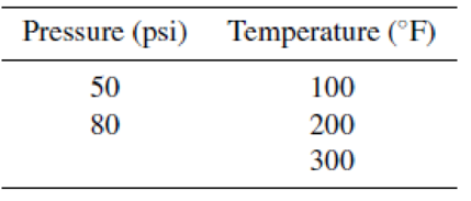
One run of the experiment at each temperature–pressure combination gave the data listed in the following table.
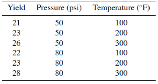
a Fit the model
b Test to see whether β3 differs significantly from zero, with α = .05.
c Test the hypothesis that temperature does not affect the yield, with α = .05.
Want to see the full answer?
Check out a sample textbook solution
Chapter 11 Solutions
Mathematical Statistics with Applications


- The owner of a new car conducts a series of six gas mileage tests and obtains the following results, expressed in miles per gallon: 3., 22.7, 21.4, 20.6, and 21.4. 20.9. Find the mode for these data.arrow_forwardA sociologist wants to determine if the life expectancy of people in Africa is less than the life expectancy of people in Asia. The data obtained is shown in the table below. Africa Asia = 63.3 yr. 1 X,=65.2 yr. 2 o, = 9.1 yr. = 7.3 yr. n1 = 120 = 150arrow_forwardThe following data refers to yield of tomatoes (kg/plot) for four different levels of salinity. Salinity level here refers to electrical conductivity (EC), where the chosen levels were EC = 1.6, 3.8, 6.0, and 10.2 nmhos/cm. (Use i = 1, 2, 3, and 4 respectively.) 1.6: 59.4 53.4 56.3 63.2 58.4 3.8: 55.9 59.7 52.7 54.2 6.0: 51.7 48.2 53.9 49.0 10.2: 44.3 48.3 40.7 47.2 46.7 W23 = W 24 = W34 = USE SALT Apply the modified Tukey's method to identify significant differences among us. (Round your answers to two decimal places.) W12 = W13 = W14= Which pairs are significantly different? (Select all that apply.) Othe group and the 3.8 group the 1.6 group and the 6.0 group the 1.6 group and the 10.2 group the 3.8 group and the 6.0 group the 3.8 group and the 10.2 group O the 6.0 group and the 10.2 group There are no significant differences.arrow_forward
- Show solution, do not use excel 1. A study was conducted to compare three methods of measuring concentration of certain type of chemical pollutants in a lake. The data is given in Table 1 below. a. Compute SS(between) and SS(within). b. Compute SS(total), and explain the relationship between SS(between), SS(within), and SS(total). c. Compute MS(between), MS(within), and F statistic. d. Based on your computations, are there significant differences in the mean pollutant concentrations among the three methods? Table 1. Amount of concentration of a chemical pollutant in a lake using three different measuring methods Method 1 Method 2 Method 3 10.96 10.88 10.73 10.75 10.80 10.77 10.79 10.90 10.78 10.82 10.69 10.81 10.87 10.70 10.88 10.6 10.82 10.81arrow_forwardWe are interested in using the pH of the lake water (which is easy to measure) to predict the average mercury level in fish from the lake, which is hard to measure. Let x be the pH of the lake water and Y be the average mercury level in fish from the lake. A sample of n = 10 lakes yielded the following data: Observation (i) pH (x;) Average mercury level (y;) 1 3 6 7 9 10 8.2 8.4 7.0 7.2 7.3 6.4 9.1 5.8 7.6 8.1 0.15 0.04 0.40 0.50 0.27 0.81 0.04 0.83 0.05 0.19 Suppose we fit the data with the following regression model: Y; = a+ Bx; + Ei, i = 1, ... , 10, where ɛ; ~ N(0, o²) are independent. We have the following quantities: a = E1 ; = 7.51, j = £i=1 Yi = 0.328, E1 x? = 572.71, 1 y? = 1.8922, -1 Tiyi = 22.218. n i=1 Some R output that may help. > p1 qt (p1, 8) [1] -2.896 -2.306 -1.860 -1.397 > qt (p1, 9) [1] -2.821 -2.262 -1.833 -1.383 1.397 1.860 2.306 2.896 1.383 1.833 2.262 2.821 (a) Find the ordinary least squares (OLS) estimates (denoted as â and B) of the regression coefficients…arrow_forwardWe are interested in using the pH of the lake water (which is easy to measure) to predict the average mercury level in fish from the lake, which is hard to measure. Let x be the pH of the lake water and Y be the average mercury level in fish from the lake. A sample of n = 10 lakes yielded the following data: Observation (i) pH (x;) Average mercury level (y;) 0.15 1 3 4 6 7 8 9 10 8.2 8.4 7.0 7.2 7.3 6.4 9.1 5.8 7.6 8.1 0.04 0.40 0.50 0.27 0.81 0.04 0.83 0.05 0.19 Suppose we fit the data with the following regression model: Y; = a + Bx; + Ei, i = 1, ..., 10, where ɛi ~ N (0, o?) are independent. We have the following quantities: a = E=1 ¤i = 7.51, j = E1 Yi = 0.328, 1 x = 572.71, 1 Y? = 1.8922, D-1 *iYi = 22.218. i=1 ri=1 Some R output that may help. > р1 qt (p1, 8) [1] -2.896 -2.306 -1.860 -1.397 1.397 1.860 2.306 2.896 > qt (p1, 9) [1] -2.821 -2.262 -1.833 -1.383 1.383 1.833 2.262 2.821 (a) Find the ordinary least squares (OLS) estimates (denoted as â and ß) of the regression…arrow_forward
- An experiment was conducted to study the extrusion process of biodegradable packaging foam. Two of the factors considered for their effect on the foam diameter (mm) were the die temperature(145°C vs.155°C) and the die diameter (3 mm vs. 4 mm). The results are in the accompanying data table. The question are attached in a photoarrow_forwardThe following data refers to yield of tomatoes (kg/plot) for four different levels of salinity. Salinity level here refers to electrical conductivity (EC), where the chosen levels were EC = 1.6, 3.8, 6.0, and 10.2 nmhos/cm. (Use i = 1, 2, 3, and 4 respectively.) 1.6: 59.3 53.9 56.5 63.1 58.6 3.8: 55.4 59.9 52.2 54.6 6.0: 51.2 48.3 53.1 48.9 10.2: 44.7 48.2 41.1 47.1 46.9 Use the F test at level a = 0.05 to test for any differences in true average yield due to the different salinity levels. State the appropriate hypotheses. Hạ: at least two us are equal O Ho: H = z = 43 = Ha H: all four u,'s are unequal O Ho: H = uz = H3 - Ha Hạ: at least two 4's are unequal H: all four u,'s are equal Calculate the test statistic. (Round your answer to two decimal places.)arrow_forwardThe following data refers to yield of tomatoes (kg/plot) for four different levels of salinity. Salinity level here refers to electrical conductivity (EC), where the chosen levels were EC = 1.6, 3.8, 6.0, and 10.2 nmhos/cm. (Use i = 1, 2, 3, and 4 respectively.) 1.6: 59.9 53.5 56.7 63.2 58.6 3.8: 55.6 59.6 52.6 54.5 6.0: 51.2 48.6 53.8 48.9 10.2: 44.3 48.4 41.0 47.9 46.5 In USE SALT Use the F test at level a = 0.05 to test for any differences in true average yield due to the different salinity levels. State the appropriate hypotheses. O Ho: H1 = H2 = !3 = H4 H: all four u's are unequal O Ho: H1 = H2 = H3 = H4 H: at least two u's are unequal O Ho: H1 # Hq # Hz# H4 H: all four u's are equal O Ho: H1* H2 * H3# H4 H: at least two u's are equal Calculate the test statistic. (Round your answer to two decimal places.) f = What can be said about the P-value for the test? O P-value > 0.100 O 0.050 < p-value < 0.100 O 0.010 < p-value < 0.050 O 0.001 < P-value < 0.010 O P-value < 0.001arrow_forward
- The following data refers to yield of tomatoes (kg/plot) for four different levels of salinity. Salinity level here refers to electrical conductivity (EC), where the chosen levels were EC = 1.6, 3.8, 6.0, and 10.2 nmhos/cm. (Use i = 1, 2, 3, and 4 respectively.) 1.6: 59.1 53.1 56.9 63.8 58.1 3.8: 55.6 59.1 52.8 54.1 6.0: 51.6 48.6 53.5 49.2 10.2: 44.7 48.9 40.9 47.5 46.5 Calculate the test statistic. (Round your answer to two decimal places.)arrow_forwardIn your Capstone software create a table with the following variables: Position x, m: 1, 2, 3, 4 Coefficient of friction μ: 0.36 Velocity v, m/s: v=V 2. u.9.8.xarrow_forwardThe following data represent partial pressure of CO2 and the related respiration rates for males and females. Provide a research quality analysis of these data. Show all steps. Please justify your choice of analysisarrow_forward
