
Concept explainers
Videos
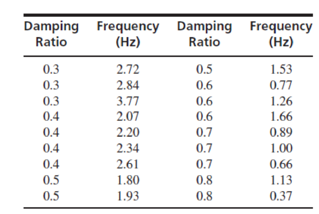
Structural engineers use wireless sensor networks to monitor the condition of dams and bridges. The article “Statistical Analysis of Vibration
- a. Construct a
scatterplot of frequency (y) versus damping ratio (x). Verify that a linear model is appropriate. - b. Compute the least-squares line for predicting frequency from damping ratio.
- c. If two modes differ in damping ratio by 0.2, by how much would you predict their frequencies to differ?
- d. Predict the frequency for modes with damping ratio 0.75.
- e. Should the equation be used to predict the frequency for modes that are overdamped (damping ratio > 1)? Explain why or why not.
- f. For what damping ratio would you predict a frequency of 2.0?
Want to see the full answer?
Check out a sample textbook solution
Chapter 7 Solutions
Statistics for Engineers and Scientists
Additional Math Textbook Solutions
Statistical Reasoning for Everyday Life (5th Edition)
Fundamentals of Statistics (5th Edition)
Business Analytics
Research Methods for the Behavioral Sciences (MindTap Course List)
Elementary Statistics Using The Ti-83/84 Plus Calculator, Books A La Carte Edition (5th Edition)


- Structural engineers use wireless sensor networks to monitor the condition of dams and bridges. The article “Statistical Analysis of Vibration Modes of a Suspension Bridge Using Spatially Dense Wireless Sensor Network" (S. Pakzad and G. Fenves, Journal of Structural Engineering, 2009:863-872) describes an experiment in which accelerometers were placed on the Golden Gate Bridge for the purpose of estimating vibration modes. The following output (from MINITAB) describes the fit of a linear model that predicts the frequency (in Hz) in terms of the damping ratio for overdamped (damping ratio > 1) modes. There are n = 7 observations. The regression equation is Frequency = 0.773 - 0.280 Damping Ratio Predictor Coef SE Coef Constant 0.77289 0.14534 5.31760.003 Damping -0.279850.079258 -3.53090.017 Ratio How many degrees of freedom are there for the Student's t statistics? Find a 98% confidence interval for ß1. a. b. Find a 98% confidence interval for Bo- C. d. Someone claims that the…arrow_forwardFoot ulcers are a common problem for people with diabetes. Higher skin temperatures on the foot indicate an increased risk of ulcers. The article "An Intelligent Insole for Diabetic Patients with the Loss of Protective Sensation" (Kimberly Anderson, M.S. Thesis, Colorado School of Mines), reports measurements of temperatures, in °F, of both feet for 181 diabetic patients. The results are presented in the following table. Left Foot Right Foot 80 80 85 85 75 80 88 86 89 87 87 82 78 78 88 89 89 90 76 81 89 86 87 82 78 78 80 81 87 82 86 85 76 80 88 89 Construct a scatterplot of the right foot temperature (y) versus the left foot temperature (x). Verify that a linear model is appropriate. b. Compute the least-squares line for predicting the right foot temperature from the left foot temperature. If the left foot temperatures of two patients differ by 2 degrees, by how much would you predict their right foot temperatures to differ? Predict the right foot temperature for a patient whose left…arrow_forwardThe article in the ASCE Journal of Energy Engineering (1999, Vol. 125, pp.59-75) describes a study of the thermal inertia properties of autoclaved aerated concrete used as a building material. Five samples of the material were tested in a structure, and the average interior temperatures (°C) reported were as follows: 23.01, 22.22, 22.04, 22.62, and 22.59. Test that the average interior temperature is equal to 22.5°C using alpha (a) = 0.05. This problem is a test on what population parameter? What is the null and alternative hypothesis? What are the Significance level and type of test? What standardized test statistic will be used? What is the standard test statistic? What is the Statistical Decision? What is the statistical decision in the statement form?arrow_forward
- 5) Alcohol consumption is influenced by price and packaging, but what about glassware? Atwood et al. (2012) measured whether the time taken to drink a beer was influenced by the shape of the glass in which it was served. Participants were given a 12 oz. of chilled lager and were told that they should drink it at their own pace while watching a nature documentary. The participants were randomly assigned to receive their beer in either a straight-sided glass or a curved, fluted glass. The data below are the total time in minutes to drink the glass of beer by the 19 women participants in the study. Straight glass: 11.63 10.37 17.89 6.96 20.40 20.64 9.26 18.11 10.33 23.54 Curved glass: 7.46 9.28 8.90 6.73 8.25 6.16 13.09 2.10 6.37 a. Show the data in a graph. What trend is suggested? Comment on other differences between the frequency distributions of the two samples. b. Test whether the mean total time to drink the beer differs depending on beer glass shape.arrow_forwardBody Fat. In the paper “Total Body Composition by Dual- Photon (153 Gd) Absorptiometry” (American Journal of Clinical Nutrition, Vol. 40, pp. 834–839), R. Mazess et al. studied methods for quantifying body composition. Eighteen randomly selected adults were measured for percentage of body fat, using dual-photon absorptiometry. Each adult’s age and percentage of body fat are shown on the WeissStats site. a. Decide whether you can reasonably apply the regression t-test. If so, then also do part (b). b. Decide, at the 5% significance level, whether the data provide sufficient evidence to conclude that the predictor variable is useful for predicting the response variable.arrow_forwardBody Fat. In the paper “Total Body Composition by Dual- Photon (153 Gd) Absorptiometry” (American Journal of Clinical Nutrition, Vol. 40, pp. 834–839), R. Mazess et al. studied methods for quantifying body composition. Eighteen randomly selected adults were measured for percentage of body fat, using dual-photon absorptiometry. Each adult’s age and percentage of body fat are shown on the WeissStats site. a. Decide whether finding a regression line for the data is reasonable. If so, then also do parts (b)–(d). b. Obtain the coefficient of determination. c. Determine the percentage of variation in the observed values of the response variable explained by the regression, and interpret your answer. d. State how useful the regression equation appears to be for making predictions.arrow_forward
- The article “Approximate Methods for Estimating Hysteretic Energy Demand on PlanAsymmetric Buildings” (M. Rathhore, A. Chowdhury, and S. Ghosh, Journal of Earthquake Engineering, 2011: 99–123) presents a method, based on a modal pushover analysis, of estimating the hysteretic energy demand placed on a structure by an earthquake. A sample of 18 measurements had a mean error of 457.8 kNm with a standard deviation of 317.7 kNm. An engineer claims that the method is unbiased, in other words, that the mean error is 0. Can you conclude that this claim is false?arrow_forwardFoot ulcers are common problem for people with diabetes. Higher skin temperatures on the foot indicate an increased risk of ulcers. The article “An Intelligent Insole for Diabetic Patients with the Loss of Protective Sensation" (Kimberly Anderson, M.S. Thesis, Colorado School of Mines), reports measurements of temperatures, in °F, of both feet for 18 diabetic patients. The results are presented in the Table QI. Table Q1: Measurements of temperatures, in °F of left foot Vs right foot for 18 diabetic patients Left Foot 80 foo Right Foot Right Foot 81 Left Foot (a) berature m80 85 76 85 89 86 9 marks) 75 80 87 82 88 foot temper 86sof 89 would thei 87 ht foo temp 80ures will 78s differ by 278reespredict by 81 (b) 87 82 87 82 I marks) 78 right foot to9erature for 76 tient whose 0 foot tmperature 78 86 85 (c) 88 89 90 88 89 (I marks) (d) Test the slope, ß1 = 1 at 5% level of significance. (e) Calculate the coefficient of correlation r and r² and then interpret their valuesarrow_forwardCortisol is a hormone that plays an important role in mediating stress. There is a growing awareness that exposure of outdoor workers to pollutants may impact cortisol levels. The article "Plasma Cortisol Concentration and Lifestyle in a Population of Outdoor Workers" (International Journal of Environmental Health Res., 2011: 62-71) reported on a study involving three groups of police officers: 1. Traffic Police (TP) 2. Drivers (D) 3. Other Duties (0) Here is summary data on cortisol concentration (ng/ml) for a subset of the officers who neither drank nor smoked. Group Sample Size Mean SD TP 174.7 50.9 160.2 37.2 153.5 45.9 44 44 44 Assuming that the standard assumptions for one-way ANOVA are satisfied, carry out a test at significance level 0.05 to decide whether the true average cortisol concentration is different for the three groups. If any differences exist, state which groups are different.arrow_forward
- The authors of the paper "Statistical Methods for Assessing Agreement Between Two Methods of Clinical Measurement" compared two different instruments for measuring a subject's ability to breathe out air.+ (This measurement is helpful in diagnosing various lung disorders.) The two instruments considered were a Wright peak flow meter and a mini-Wright peak flow meter. Seventeen subjects participated in the study, and for each subject air flow was measured once using the Wright meter and once using the mini-Wright meter. Mini- Subject Wright Meter 1 2 3 4 5 6 7 8 9 512 430 520 428 500 600 364 380 658 Wright Meter 494 395 516 434 476 557 413 442 650 Subject 10 11 12 13 14 15 16 17 Mini- Wright Meter 445 432 626 260 477 259 350 451 Wright Meter 433 417 656 267 478 178 423 427 (a) Suppose that the Wright meter is considered to provide a better measure of air flow, but the mini-Wright meter is easier to transport and to use. If the two types of meters produce different readings but there is a…arrow_forwardWhen the light turns yellow, should you stop or go through it? The article “Evaluation of Driver Behavior in Type II Dilemma Zones at High-Speed Signalized Intersections” (D. Hurwitz, M. Knodler, and B. Nyquist, Journal of Transportation Engineering, 2011:277– 286) defines the “indecision zone” as the period when a vehicle is between 2.5 and 5.5 seconds away from an intersection. It presents observations of 710 vehicles passing through various intersections in Vermont for which the light turned yellow in the indecision zone. Of the 710 vehicles, 89 ran a red light. a) Find a 90% confidence interval for the proportion of vehicles that will run the red light when encountering a yellow light in the indecision zone. b) Find a 95% confidence interval for the proportion of vehicles that will run the red light when encountering a yellow light in the indecision zone. c) Find a 99% confidence interval for the proportion of vehicles that will run the red light when encountering a yellow light in…arrow_forwardThe article "Refinement of Gravimetric Geoid Using GPS and Leveling Data" (W. Thurston, Journal of Surveying Engineering, 2000:27-56) presents a method for measuring orthometric heights above sea level. For a sample of 1225 baselines, 926 gave results that were within the class C spirit leveling tolerance limits. Can we conclude that this method produces results within the tolerance limits more than 75% of the time? Test on a 5% significance level. The P-value is 0.32, we cannot conclude that the method produces good results more than 75% of the time. The P-value is 0.01, we can conclude that the method produces good results more than 75% of the time. The P-value is 0.03, we can conclude that the method produces good results more than 75% of the time. The P-value is 0.27, we cannot conclude that the method produces good results more than 75% of the time.arrow_forward
 MATLAB: An Introduction with ApplicationsStatisticsISBN:9781119256830Author:Amos GilatPublisher:John Wiley & Sons Inc
 Probability and Statistics for Engineering and th...StatisticsISBN:9781305251809Author:Jay L. DevorePublisher:Cengage Learning
 Statistics for The Behavioral Sciences (MindTap C...StatisticsISBN:9781305504912Author:Frederick J Gravetter, Larry B. WallnauPublisher:Cengage Learning
 Elementary Statistics: Picturing the World (7th E...StatisticsISBN:9780134683416Author:Ron Larson, Betsy FarberPublisher:PEARSON
 The Basic Practice of StatisticsStatisticsISBN:9781319042578Author:David S. Moore, William I. Notz, Michael A. FlignerPublisher:W. H. Freeman
 Introduction to the Practice of StatisticsStatisticsISBN:9781319013387Author:David S. Moore, George P. McCabe, Bruce A. CraigPublisher:W. H. Freeman