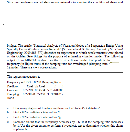
Structural engineers use wireless sensor networks to monitor the condition of dams andbridges. The article “Statistical Analysis of Vibration Modes of a Suspension Bridge UsingSpatially Dense Wireless Sensor Network" (S. Pakzad and G. Fenves, Journal of StructuralEngineering, 2009:863-872) describes an experiment in which accelerometers were placedon the Golden Gate Bridge for the purpose of estimating vibration modes. The followingoutput (from MINITAB) describes the fit of a linear model that predicts thefrequency (in Hz) in terms of the damping ratio for overdamped (damping ratio >1) modes. There are n = 7 observations.The regression equation isFrequency = 0.773 - 0.280 Damping RatioPredictorCoef SE CoefConstant0.77289 0.14534 5.31760.003Damping -0.279850.079258 -3.53090.017RatioHow many degrees of freedom are there for the Student's t statistics?Find a 98% confidence interval for ß1.a.b.Find a 98% confidence interval for Bo-C.d.Someone claims that the frequency decreases by 0.6 Hz if the damping ratio increasesby 1. Use the given output to perform a hypothesis test to determine whether this claimis plausible.

Answered: Image /qna-images/answer/395fab74-4e48-4193-a784-84166e21deb7.jpg

Answered: Structural engineers use wireless…

MATLAB: An Introduction with Applications

6th Edition

ISBN:9781119256830

Author:Amos Gilat

Publisher:Amos Gilat

Chapter1: Starting With Matlab

Section: Chapter Questions

Problem 1P

See similar textbooks

Similar questions

2. Five 2 cm thick experimental pieces of an insulation material were tested atrandom. Resulted compression (y) was measured recorded for the given amount ofmeasured pressure. The data are listed below:Pressure Compression1 12 23 24 35 5Fit a simple linear model relating compression y to the applied pressure x and find:a) error variance.b) the coefficient of correlation.
In a study examining the effect of alcohol on reaction time, Liguori and Robinson (2001) found that evenmoderate alcohol consumption significantly slowed response time to an emergency situation in a drivingsimulation. In a similar study, researchers measured reaction time 30 minutes after participants consumed one6-ounce glass of wine. Again, they used a standardized driving simulation task for which the regular populationaverages μ = 400 msec. The distribution of reaction times is approximately normal with σ = 40. Assume that theresearcher obtained a sample mean of M = 422 for the n = 25 participants in the study.a. Are the data sufficient to conclude that the alcohol has a significant effect on reaction time? Use a two-tailed testwith α = .01.
A state agency requires a minimum of 5 parts per million (ppm) of dissolved oxygen in order for the oxygen content to be sufficient to support aquatic life. Six water specimens taken from a river at a specific location during the low-water season (July) gave readings of 4.8, 5.2, 4.8, 4.9, 4.9, and 4.6 ppm of dissolved oxygen. Do the data provide sufficient evidence to indicate that the dissolved oxygen content is less than 5 ppm? Test using ? = 0.05. a) state null and alternate hypotheses b) state the test statistic c) state the rejection region d) state the conclusion
The following table shows the typical depth (rounded to the nearest foot) for nonfailed wells in geological formations in Baltimore County (The Journal of Data Science, 2009, Vol. 7, pp. 111-127). Geological Formation Group Number of Nonfailed Wells Nonfailed Well Depth Gneiss 1,515 255 Granite 26 218 Loch Raven Schist 3,290 317 Mafic 349 231 Marble 280 267 Prettyboy Schist 1,343 255 Other schists 887 267 Serpentine 36 217 Total 7,726 2,027 Let the random variable X denote the depth (rounded to the nearest foot) for nonfailed wells. Detemine the cumulative distribution function for X. Round your answers to four decimal places (e.g. 98.7654). x < 217 217
Refer to Exercise 8.S.6. Analyze these data using a Wilcoxon signed-rank test.
The article "Secretion of Parathyroid Hormone Oscillates Depending on the Change in Serum Ionized Calcium During Hemodialysis and May Affect Bone Metabolism" (T. Kitahara, K. Ueki, et al., Nephron Clinical Practice, 2005: c9-c17) presents measurements of basal ionized calcium (Ca) levels for four groups of patients with differing levels of basal intact parathyroid hormone (PTH). The following results are consistent with means and standard deviations presented in the article. Group Ca levels (mM) I 1.23 1.02 1.33 1.36 1.11 1.51 1.51 1.30 1.36 1.34 1.27 1.43 1.21 1.69 1.33 1.49 II 1.18 1.16 1.07 1.21 1.01 1.26 1.37 1.09 1.28 1.33 0.98 0.99 1.24 1.12 1.27 1.26 1.33 1.26 1.32 III 1.04 1.32 1.29 0.95 1.38 1.08 1.65 1.14 1.44 1.37 1.11 0.82 1.31 1.09 IV 1.35 1.67 1.38 1.05 1.32 0.95 1.21 1.21 1.22 1.13 1.51 0.72 1.33 1.46 Construct an ANOVA table. You may give a range for the P-value. Can you conclude that there are differences among the mean Ca levels? a. b.
Following are measurements of soil concentrations (in mg /kg) of chromium (Cr) and nickel (Ni) at20 sites in the area of Cleveland, Ohio. These data are taken from the article "Variation in NorthAmerican Regulatory Guidance for Heavy Metal Surface Soil Contamination at Commercial andIndustrial Sites" (A. Jennings and J. Ma, J. Environment Eng, 2007:587-609). Cr: 260 19 36 247 263 319 317 277 319 264 23 29 61 119 33 281 21 35 64 30Ni: 435 377 359 53 38 38 54 188 397 33 92 490 28 35 799 347 321 32 74 508 (a) Construct a histogram for each set of concentrations. (b) Find the 1st, 2nd and 3rd quartiles for the Cr concentrations (c) Find the 1st, 2nd and 3rd quartiles for the Ni concentrations.
Neurosurgery Operative Times. An Arizona State University professor, R. Jacobowitz, Ph.D., in consultation with G. Vishteh, M.D., and other neurosurgeons obtained data on operative times, in minutes, for both a dynamic system (Z-plate) and a static system (ALPS plate). They wanted to perform a hypothesis test to decide whether the mean operative time is less with the dynamic system than with the static system. a. identify the variable. b. identify the two populations. c. determine the null and alternative hypotheses. d. classify the hypothesis test as two tailed, left tailed, or right tailed.
The decline of salmon fisheries along the Columbia River in Oregon has caused great concern among commercial and recreational fishermen. The paper 'Feeding of Predaceous Fishes on Out-Migrating Juvenile Salmonids in John Day Reservoir, Columbia River' (Trans. Amer. Fisheries Soc. (1991: 405-420) gave the accompanying data on y = maximum size of salmonids consumed by a northern squaw fish (the most abundant salmonid predator) and x = squawfish length, both in mm. Here is the computer software printout of the summary: Coefficients: Estimate Std. Error t value Pr(> |t|) (Intercept) −89.010 16.703 −5.329 0.000 Length 0.705 0.046 15.293 0.000 Using this information, give the equation of the least squares regression line.
NW 6.12 CORPORATE SUSTAINABILITY OF CPA FIRMS. Corporate sustainability refers to business practices designed CORSUS around social and environmental considerations. Refer to the Business and Society (March 2011) study on the sustainability behaviors of CPA corporations, Exercise 2.23 (p. 59). Recall that the level of support for corporate sustainability (measured on a quantitative scale ranging from 0 to 160 points) was obtained for each in a sample of 992 senior managers at CPA firms. Higher point values indicate a higher level of support for sustainability. The accompanying StatCrunch printout gives a 99% confidence interval for the mean level of support for all senior managers at CPA firms. One sample T confidence interval: μ: Mean of variable 99% confidence interval results: Variable Sample Mean Std. Err. DF L. Limit U. Limit Support 67.75504 0.85314633 991 65.553241 69.95684 a. Locate the 99% confidence interval on the printout. b. Use the sample mean and standard deviation on the…
The authors of the paper "Statistical Methods for Assessing Agreement Between Two Methods of Clinical Measurement"† compared two different instruments for measuring a person's ability to breathe out air. (This measurement is helpful in diagnosing various lung disorders.) The two instruments considered were a Wright peak flow meter and a mini-Wright peak flow meter. Seventeen people participated in the study, and for each person air flow was measured once using the Wright meter and once using the mini-Wright meter. Subject Mini-WrightMeter WrightMeter Subject Mini-WrightMeter WrightMeter 1 512 494 10 445 433 2 430 395 11 432 417 3 520 516 12 626 656 4 428 434 13 260 267 5 500 476 14 477 478 6 600 557 15 259 178 7 364 413 16 350 423 8 380 442 17 451 427 9 658 650 (a) Suppose that the Wright meter is considered to provide a better measure of air flow, but the mini-Wright meter is easier to transport and to use. If the two types of meters produce…
If you had four factors, were interested in main effects and two-way interactions and wanted to conduct a three-level Central Composite Design, the total experimental runs would be the coded axial value would be ? and

Recommended textbooks for you

MATLAB: An Introduction with Applications

Statistics

ISBN:

9781119256830

Author:

Amos Gilat

Publisher:

John Wiley & Sons Inc

Probability and Statistics for Engineering and th…

Statistics

ISBN:

9781305251809

Author:

Jay L. Devore

Publisher:

Cengage Learning

Statistics for The Behavioral Sciences (MindTap C…

Statistics

ISBN:

9781305504912

Author:

Frederick J Gravetter, Larry B. Wallnau

Publisher:

Cengage Learning

MATLAB: An Introduction with Applications

Statistics

ISBN:

9781119256830

Author:

Amos Gilat

Publisher:

John Wiley & Sons Inc

Probability and Statistics for Engineering and th…

Statistics

ISBN:

9781305251809

Author:

Jay L. Devore

Publisher:

Cengage Learning

Statistics for The Behavioral Sciences (MindTap C…

Statistics

ISBN:

9781305504912

Author:

Frederick J Gravetter, Larry B. Wallnau

Publisher:

Cengage Learning

Elementary Statistics: Picturing the World (7th E…

Statistics

ISBN:

9780134683416

Author:

Ron Larson, Betsy Farber

Publisher:

PEARSON

The Basic Practice of Statistics

Statistics

ISBN:

9781319042578

Author:

David S. Moore, William I. Notz, Michael A. Fligner

Publisher:

W. H. Freeman

Introduction to the Practice of Statistics

Statistics

ISBN:

9781319013387

Author:

David S. Moore, George P. McCabe, Bruce A. Craig

Publisher:

W. H. Freeman

SEE MORE TEXTBOOKS