
Statistics for Engineers and Scientists
4th Edition
ISBN: 9780073401331
Author: William Navidi Prof.
Publisher: McGraw-Hill Education
expand_more
expand_more
format_list_bulleted
Concept explainers
Videos
Textbook Question
Chapter 7.4, Problem 1E
The following output (from MINITAB) is for the least-squares fit of the model ln y = β0 + β1 ln x + ε, where y represents the monthly production of a gas well and x represents the volume of fracture fluid pumped in. (A
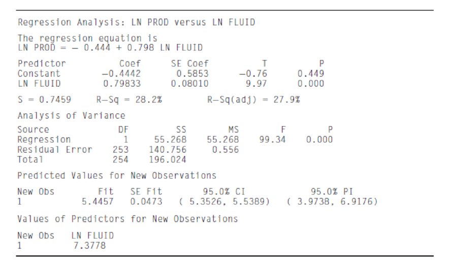
- a. What is the equation of the least-squares line for predicting ln y from ln x?
- b. Predict the production of a well into which 2500 gal/ft of fluid have been pumped.
- c. Predict the production of a well into which 1600 gal/ft of fluid have been pumped.
- d. Find a 95% prediction interval for the production of a well into which 1600 gal/ft of fluid have been pumped. (Note: In 1600 = 7.3778.)
Expert Solution & Answer
Want to see the full answer?
Check out a sample textbook solution
Students have asked these similar questions
5. The relationship between the number of beers consumed (x) and the blood alcohol
content (v) was studied in 20 male students using the least squares regression. The
following regression model (equation), was obtained from the study:
y = 0.0127 +0.0180x. This equation implies that:
a. Each beer consumed increases blood alcohol by 1.27%
b. On average it takes 1.8 beers to increase blood alcohol content by 1%
c. Each beer consumed increases blood alcohol level by 0.018
d. Each beer consumed increases blood alcohol by an average amount of 1.8%
The following estimated regression equation was developed for a model involving two independent variables.
ý = 40.7 + 8.63x, + 2.71.x,
After x 2 was dropped from the model, the least squares method was used to obtain an estimated regression equation involving only
X 1 as an independent variable.
ŷ = 42.0 + 9.01x
a. In the two independent variable case, the coefficient x 1 represents the expected change in Select v corresponding to a one unit
increase in Select v when Select v is held constant.
In the single independent variable case, the coefficient x 1 represents the expected change in Select v corresponding to a one
unit increase in Select v
b. Could multicollinearity explain why the coefficient of x 1 differs in the two models? Assume that x1 and x2 are correlated.
Select
The relationship between number of beers consumed (x) and blood alcohol content (y) was studied in 16 male college students by using least squares regression. The following regression equation was obtained from this study: y-hat = -0.0127 + 0.0180x The above equation implies that:
each beer consumed increases blood alcohol by .0127
on average it takes 1.8 beers to increase blood alcohol content by .01
After consuming 1 beer, blood alcohol equals .0180.
each beer consumed increases blood alcohol by 0.018
Chapter 7 Solutions
Statistics for Engineers and Scientists
Ch. 7.1 - Compute the correlation coefficient for the...Ch. 7.1 - For each of the following data sets, explain why...Ch. 7.1 - For each of the following scatterplots, state...Ch. 7.1 - True or false, and explain briefly: a. If the...Ch. 7.1 - In a study of ground motion caused by earthquakes,...Ch. 7.1 - A chemical engineer is studying the effect of...Ch. 7.1 - Another chemical engineer is studying the same...Ch. 7.1 - Tire pressure (in kPa) was measured for the right...Ch. 7.1 - Prob. 10ECh. 7.1 - The article Drift in Posturography Systems...
Ch. 7.1 - Prob. 12ECh. 7.1 - Prob. 13ECh. 7.1 - A scatterplot contains four points: (2, 2), (1,...Ch. 7.2 - Each month for several months, the average...Ch. 7.2 - In a study of the relationship between the Brinell...Ch. 7.2 - A least-squares line is fit to a set of points. If...Ch. 7.2 - Prob. 4ECh. 7.2 - In Galtons height data (Figure 7.1, in Section...Ch. 7.2 - In a study relating the degree of warping, in mm....Ch. 7.2 - Moisture content in percent by volume (x) and...Ch. 7.2 - The following table presents shear strengths (in...Ch. 7.2 - Structural engineers use wireless sensor networks...Ch. 7.2 - The article Effect of Environmental Factors on...Ch. 7.2 - An agricultural scientist planted alfalfa on...Ch. 7.2 - Curing times in days (x) and compressive strengths...Ch. 7.2 - Prob. 13ECh. 7.2 - An engineer wants to predict the value for y when...Ch. 7.2 - A simple random sample of 100 men aged 2534...Ch. 7.2 - Prob. 16ECh. 7.3 - A chemical reaction is run 12 times, and the...Ch. 7.3 - Structural engineers use wireless sensor networks...Ch. 7.3 - Prob. 3ECh. 7.3 - Prob. 4ECh. 7.3 - Prob. 5ECh. 7.3 - Prob. 6ECh. 7.3 - The coefficient of absorption (COA) for a clay...Ch. 7.3 - Prob. 8ECh. 7.3 - Prob. 9ECh. 7.3 - Three engineers are independently estimating the...Ch. 7.3 - In the skin permeability example (Example 7.17)...Ch. 7.3 - Prob. 12ECh. 7.3 - In a study of copper bars, the relationship...Ch. 7.3 - Prob. 14ECh. 7.3 - In the following MINITAB output, some of the...Ch. 7.3 - Prob. 16ECh. 7.3 - In order to increase the production of gas wells,...Ch. 7.4 - The following output (from MINITAB) is for the...Ch. 7.4 - The processing of raw coal involves washing, in...Ch. 7.4 - To determine the effect of temperature on the...Ch. 7.4 - The depth of wetting of a soil is the depth to...Ch. 7.4 - Good forecasting and control of preconstruction...Ch. 7.4 - The article Drift in Posturography Systems...Ch. 7.4 - Prob. 7ECh. 7.4 - Prob. 8ECh. 7.4 - A windmill is used to generate direct current....Ch. 7.4 - Two radon detectors were placed in different...Ch. 7.4 - Prob. 11ECh. 7.4 - The article The Selection of Yeast Strains for the...Ch. 7.4 - Prob. 13ECh. 7.4 - The article Characteristics and Trends of River...Ch. 7.4 - Prob. 15ECh. 7.4 - The article Mechanistic-Empirical Design of...Ch. 7.4 - An engineer wants to determine the spring constant...Ch. 7 - The BeerLambert law relates the absorbance A of a...Ch. 7 - Prob. 2SECh. 7 - Prob. 3SECh. 7 - Refer to Exercise 3. a. Plot the residuals versus...Ch. 7 - Prob. 5SECh. 7 - The article Experimental Measurement of Radiative...Ch. 7 - Prob. 7SECh. 7 - Prob. 8SECh. 7 - Prob. 9SECh. 7 - Prob. 10SECh. 7 - The article Estimating Population Abundance in...Ch. 7 - A materials scientist is experimenting with a new...Ch. 7 - Monitoring the yield of a particular chemical...Ch. 7 - Prob. 14SECh. 7 - Refer to Exercise 14. Someone wants to compute a...Ch. 7 - Prob. 16SECh. 7 - Prob. 17SECh. 7 - Prob. 18SECh. 7 - Prob. 19SECh. 7 - Use Equation (7.34) (page 545) to show that 1=1.Ch. 7 - Use Equation (7.35) (page 545) to show that 0=0.Ch. 7 - Prob. 22SECh. 7 - Use Equation (7.35) (page 545) to derive the...
Additional Math Textbook Solutions
Find more solutions based on key concepts
Use the model developed in Example 1.5 to predict the total sales for weeks 2 through 16, and compare the resul...
Business Analytics
Teacher Salaries
The following data from several years ago represent salaries (in dollars) from a school distri...
Elementary Statistics: A Step By Step Approach
Teacher Salaries
The following data from several years ago represent salaries (in dollars) from a school distri...
Elementary Statistics: A Step By Step Approach
Refer to the Real Estate data, which reports information on homes sold in the Goodyear, Arizona, area during th...
Statistical Techniques in Business and Economics
Medication Usage In a survey of 3005 adults aged 57 through 85 years, it was found that 82% of them used at lea...
Statistical Reasoning for Everyday Life (5th Edition)
TRY IT YOURSELF 2
Determine whether each number describes a population parameter or a sample statistic. Explain...
Elementary Statistics: Picturing the World (7th Edition)
Knowledge Booster


Learn more about
Need a deep-dive on the concept behind this application? Look no further. Learn more about this topic, statistics and related others by exploring similar questions and additional content below.Similar questions
- Respiratory Rate Researchers have found that the 95 th percentile the value at which 95% of the data are at or below for respiratory rates in breath per minute during the first 3 years of infancy are given by y=101.82411-0.0125995x+0.00013401x2 for awake infants and y=101.72858-0.0139928x+0.00017646x2 for sleeping infants, where x is the age in months. Source: Pediatrics. a. What is the domain for each function? b. For each respiratory rate, is the rate decreasing or increasing over the first 3 years of life? Hint: Is the graph of the quadratic in the exponent opening upward or downward? Where is the vertex? c. Verify your answer to part b using a graphing calculator. d. For a 1- year-old infant in the 95 th percentile, how much higher is the walking respiratory rate then the sleeping respiratory rate? e. f.arrow_forwardThe following table provides values of the function f(x,y). However, because of potential; errors in measurement, the functional values may be slightly inaccurately. Using the statistical package included with a graphical calculator or spreadsheet and critical thinking skills, find the function f(x,y)=a+bx+cy that best estimate the table where a, b and c are integers. Hint: Do a linear regression on each column with the value of y fixed and then use these four regression equations to determine the coefficient c. x y 0 1 2 3 0 4.02 7.04 9.98 13.00 1 6.01 9.06 11.98 14.96 2 7.99 10.95 14.02 17.09 3 9.99 13.01 16.01 19.02arrow_forwardOlympic Pole Vault The graph in Figure 7 indicates that in recent years the winning Olympic men’s pole vault height has fallen below the value predicted by the regression line in Example 2. This might have occurred because when the pole vault was a new event there was much room for improvement in vaulters’ performances, whereas now even the best training can produce only incremental advances. Let’s see whether concentrating on more recent results gives a better predictor of future records. (a) Use the data in Table 2 (page 176) to complete the table of winning pole vault heights shown in the margin. (Note that we are using x=0 to correspond to the year 1972, where this restricted data set begins.) (b) Find the regression line for the data in part ‚(a). (c) Plot the data and the regression line on the same axes. Does the regression line seem to provide a good model for the data? (d) What does the regression line predict as the winning pole vault height for the 2012 Olympics? Compare this predicted value to the actual 2012 winning height of 5.97 m, as described on page 177. Has this new regression line provided a better prediction than the line in Example 2?arrow_forward
- Find the equation of the regression line for the following data set. x 1 2 3 y 0 3 4arrow_forwardIf your graphing calculator is capable of computing a least-squares sinusoidal regression model, use it to find a second model for the data. Graph this new equation along with your first model. How do they compare?arrow_forwardThe output of a solar panel (photovoltaic) system depends on its size. A manufacturer states that the average daily production of its 1.5 kW system is 6.6 kilowatt hours (kWh) for Perth conditions. A consumer group monitored this 1.5 kW system in 20 different Perth homes and measured the average daily production by the systems in these homes over a one month period during October. The data is provided here. kWh 6.2, 5.8, 5.9, 6.1, 6.4, 6.3, 6.9, 5.5, 7.4, 6.7, 6.3, 6.2, 7.1, 6.8, 5.9, 5.4, 7.2, 6.7, 5.8, 6.9 1. Analyse the consumer group’s data to test if the manufacturer’s claim of an average of 6.6 kWh per day is reasonable. State appropriate hypotheses, assumptions and decision rule at α = 0.10. What conclusions would you report to the consumer group? (Hint: You will need to find Descriptive Statistics first.) 2. If 48 homes in the central Australian city of Alice Springs had this system installed and similar data was collected, in order to assess whether average daily production in…arrow_forward
- Solve the following statistical problems using regression analysis. 1. Regression methods were used to analyze the data from a study investigating the relationship between roadway surface temperature (x) and pavement deflection ( y). Summary quantities were n = 20. Eyi = 12.75, Eyi? = 8.86. ri = 1478. E ci? = 143, 215.80, and riyi = 1083.67. (a) Calculate the least squares estimates of the slope and intercept. Graph the regression line. (b) Use the equation of the fitted line to predict what pavement deflection would be observed when the surface temperature is 85F. (c) What is the mean pavement deflection when the surface temperature is 90F?arrow_forwardA paper gives data on x = change in Body Mass Index (BMI, in kilograms/meter2) and y = change in a measure of depression for patients suffering from depression who participated in a pulmonary rehabilitation program. The table below contains a subset of the data given in the paper and are approximate values read from a scatterplot in the paper. BMI Change (kg/m²) Depression Score Change S = The accompanying computer output is from Minitab. Depression score change 15- 10- -0.5 S Fitted Line Plot Depression score change = 6.577 +5.440 BMI change 20- 5.30586 Coefficients T 0.0 0.5 -0.5 R-sq 25.96% - 1 Term Coef Constant 6.577 BMI change 5.440 % 0.5 BMI change 1.0 SE Coef 2.28 2.90 9 0 0.1 0.7 0.8 1 1.5 4 T-Value 2.88 1.87 Interpret this estimate. s is the typical amount by which the ---Select--- line. 4 5 Regression Equation Depression score change = 6.577 +5.440 BMI change P-Value 0.0164 0.0906 S 5.30586 25.96% R-Sq R-Sq (adj) 18.56% 8 (b) Give a point estimate of o. (Round your answer to…arrow_forwardThe weight (in pounds) and height (in inches) for a child were measured every few months over a two- The equation ŷ = 17.4 + 0.5x is called the least- squares regression line because it year period. The results are displayed in the scatterplot. O is least able to make accurate predictions for the data. A Child's Weight and Height O makes the strongest association between weight and height. 40 O minimizes the sum of the squared distances from the actual y-value to the predicted y-value. 36. O maximizes the sum of the squared distances from the actual y-value to the predicted y-value. 24 20 6 8 10 12 14 16 18 20 22 24 26 28 30 32 34 36 38 40 42 Weight (Pounds) Mark this and return Save and Exit Next Subrmit rch 65°F DELL F2 F3 F4 E5 F6 F7 F8 F9 F10 F11 PriScr F12 Insert %23 %24 & 3. 4 6 8 10 W T Y 6 D F G H J K Height (Inches)arrow_forward
arrow_back_ios
arrow_forward_ios
Recommended textbooks for you
 Linear Algebra: A Modern IntroductionAlgebraISBN:9781285463247Author:David PoolePublisher:Cengage Learning
 Calculus For The Life SciencesCalculusISBN:9780321964038Author:GREENWELL, Raymond N., RITCHEY, Nathan P., Lial, Margaret L.Publisher:Pearson Addison Wesley,
 Functions and Change: A Modeling Approach to Coll...AlgebraISBN:9781337111348Author:Bruce Crauder, Benny Evans, Alan NoellPublisher:Cengage Learning
 College AlgebraAlgebraISBN:9781305115545Author:James Stewart, Lothar Redlin, Saleem WatsonPublisher:Cengage Learning
 Algebra & Trigonometry with Analytic GeometryAlgebraISBN:9781133382119Author:SwokowskiPublisher:Cengage
 Trigonometry (MindTap Course List)TrigonometryISBN:9781305652224Author:Charles P. McKeague, Mark D. TurnerPublisher:Cengage Learning
Linear Algebra: A Modern Introduction
Algebra
ISBN:9781285463247
Author:David Poole
Publisher:Cengage Learning
Calculus For The Life Sciences
Calculus
ISBN:9780321964038
Author:GREENWELL, Raymond N., RITCHEY, Nathan P., Lial, Margaret L.
Publisher:Pearson Addison Wesley,
Functions and Change: A Modeling Approach to Coll...
Algebra
ISBN:9781337111348
Author:Bruce Crauder, Benny Evans, Alan Noell
Publisher:Cengage Learning
College Algebra
Algebra
ISBN:9781305115545
Author:James Stewart, Lothar Redlin, Saleem Watson
Publisher:Cengage Learning
Algebra & Trigonometry with Analytic Geometry
Algebra
ISBN:9781133382119
Author:Swokowski
Publisher:Cengage
Trigonometry (MindTap Course List)
Trigonometry
ISBN:9781305652224
Author:Charles P. McKeague, Mark D. Turner
Publisher:Cengage Learning
Correlation Vs Regression: Difference Between them with definition & Comparison Chart; Author: Key Differences;https://www.youtube.com/watch?v=Ou2QGSJVd0U;License: Standard YouTube License, CC-BY
Correlation and Regression: Concepts with Illustrative examples; Author: LEARN & APPLY : Lean and Six Sigma;https://www.youtube.com/watch?v=xTpHD5WLuoA;License: Standard YouTube License, CC-BY