
Statistics for Engineers and Scientists
4th Edition
ISBN: 9780073401331
Author: William Navidi Prof.
Publisher: McGraw-Hill Education
expand_more
expand_more
format_list_bulleted
Concept explainers
Videos
Textbook Question
Chapter 7, Problem 13SE
Monitoring the yield of a particular chemical reaction at various reaction vessel temperatures produces the results shown in the following table.
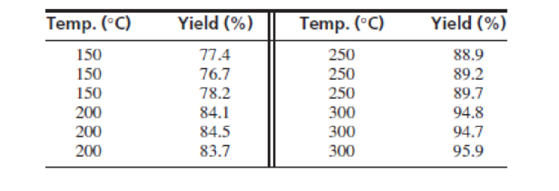
- a. Find the least-squares estimates for β0, β1, and σ2 for the simple linear model Yield = β0 + β1 Temp + ε.
- b. Can you conclude that β0 is not equal to 0?
- c. Can you conclude that β1 is not equal to 0?
- d. Make a residual plot. Does the linear model seem appropriate?
- e. Find a 95% confidence interval for the slope.
- f. Find a 95% confidence interval for the mean yield at a temperature of 225°C.
- g. Find a 95% prediction interval for a yield at a temperature of 225°C.
Expert Solution & Answer
Want to see the full answer?
Check out a sample textbook solution
Students have asked these similar questions
The relationship between the number of beers consumed and the blood alcohol content was studied in 16 male college students by using the least squares regression. The following regression equation was obtained from the study: y ̂= -0.0127+0.0180x The above equation implies that:A. each beer consumed increases blood alcohol by 1.27%.B. on the average, it takes 1.8 beers to increase blood alcohol content by 1%.C. Each beer consumed increases blood alcohol by an average amount of 1.8%.D. Each beer consumed increases blood alcohol by exactly 0.018 units.
Please answer both multiple choice questions below.
a.) A linear regression of age (x) on blood lead levels (y) is performed in a sample of men who have worked in factories that manufacture car batteries. The residual plots suggest there is still a pattern remaining, and you decide to add a cubic term for age into the model. Which of the following models is now most appropriate?
Blood lead levels = α+ β21(age) + ε, ε ~iid N(0, σ2)
Blood lead levels = α+ β1(age3) + ε2, ε ~ iid N(0, σ2)
Blood lead levels = α+ β1(age) + β2 (age2) + ε, ε ~iid N(0, σ2)
Blood lead levels = α+ β1(age) + β2 (age2) + β1 (age3) + ε, ε ~iid N(0, σ2)
b.) A study has been conducted to analyze the sensitivity and specificity of a screening test. If the area under the ROC curve is 1:
The screening test is very helpful.
The screening test is not helpful.
The screening test is somewhat helpful.
Helpfulness cannot be determined from the information given.
Let Y = β0 + β1x + E be the simple linear regression model. What is the precise interpretation of the coefficient of determination (R2)?
Select one:
a.
It is an estimate of the change in the expected value of the response variable Y for every unit increase in the explanatory variable X.
b.
It is the proportion of the variation in the response variable Y that is explained by the variation in the explanatory variable X.
c.
It is the proportion of the variation in the explanatory variable Y.
d.
It is an estimate of the change in the expected value of the response variable Y for every unit increase in the explanatory variable X.
Chapter 7 Solutions
Statistics for Engineers and Scientists
Ch. 7.1 - Compute the correlation coefficient for the...Ch. 7.1 - For each of the following data sets, explain why...Ch. 7.1 - For each of the following scatterplots, state...Ch. 7.1 - True or false, and explain briefly: a. If the...Ch. 7.1 - In a study of ground motion caused by earthquakes,...Ch. 7.1 - A chemical engineer is studying the effect of...Ch. 7.1 - Another chemical engineer is studying the same...Ch. 7.1 - Tire pressure (in kPa) was measured for the right...Ch. 7.1 - Prob. 10ECh. 7.1 - The article Drift in Posturography Systems...
Ch. 7.1 - Prob. 12ECh. 7.1 - Prob. 13ECh. 7.1 - A scatterplot contains four points: (2, 2), (1,...Ch. 7.2 - Each month for several months, the average...Ch. 7.2 - In a study of the relationship between the Brinell...Ch. 7.2 - A least-squares line is fit to a set of points. If...Ch. 7.2 - Prob. 4ECh. 7.2 - In Galtons height data (Figure 7.1, in Section...Ch. 7.2 - In a study relating the degree of warping, in mm....Ch. 7.2 - Moisture content in percent by volume (x) and...Ch. 7.2 - The following table presents shear strengths (in...Ch. 7.2 - Structural engineers use wireless sensor networks...Ch. 7.2 - The article Effect of Environmental Factors on...Ch. 7.2 - An agricultural scientist planted alfalfa on...Ch. 7.2 - Curing times in days (x) and compressive strengths...Ch. 7.2 - Prob. 13ECh. 7.2 - An engineer wants to predict the value for y when...Ch. 7.2 - A simple random sample of 100 men aged 2534...Ch. 7.2 - Prob. 16ECh. 7.3 - A chemical reaction is run 12 times, and the...Ch. 7.3 - Structural engineers use wireless sensor networks...Ch. 7.3 - Prob. 3ECh. 7.3 - Prob. 4ECh. 7.3 - Prob. 5ECh. 7.3 - Prob. 6ECh. 7.3 - The coefficient of absorption (COA) for a clay...Ch. 7.3 - Prob. 8ECh. 7.3 - Prob. 9ECh. 7.3 - Three engineers are independently estimating the...Ch. 7.3 - In the skin permeability example (Example 7.17)...Ch. 7.3 - Prob. 12ECh. 7.3 - In a study of copper bars, the relationship...Ch. 7.3 - Prob. 14ECh. 7.3 - In the following MINITAB output, some of the...Ch. 7.3 - Prob. 16ECh. 7.3 - In order to increase the production of gas wells,...Ch. 7.4 - The following output (from MINITAB) is for the...Ch. 7.4 - The processing of raw coal involves washing, in...Ch. 7.4 - To determine the effect of temperature on the...Ch. 7.4 - The depth of wetting of a soil is the depth to...Ch. 7.4 - Good forecasting and control of preconstruction...Ch. 7.4 - The article Drift in Posturography Systems...Ch. 7.4 - Prob. 7ECh. 7.4 - Prob. 8ECh. 7.4 - A windmill is used to generate direct current....Ch. 7.4 - Two radon detectors were placed in different...Ch. 7.4 - Prob. 11ECh. 7.4 - The article The Selection of Yeast Strains for the...Ch. 7.4 - Prob. 13ECh. 7.4 - The article Characteristics and Trends of River...Ch. 7.4 - Prob. 15ECh. 7.4 - The article Mechanistic-Empirical Design of...Ch. 7.4 - An engineer wants to determine the spring constant...Ch. 7 - The BeerLambert law relates the absorbance A of a...Ch. 7 - Prob. 2SECh. 7 - Prob. 3SECh. 7 - Refer to Exercise 3. a. Plot the residuals versus...Ch. 7 - Prob. 5SECh. 7 - The article Experimental Measurement of Radiative...Ch. 7 - Prob. 7SECh. 7 - Prob. 8SECh. 7 - Prob. 9SECh. 7 - Prob. 10SECh. 7 - The article Estimating Population Abundance in...Ch. 7 - A materials scientist is experimenting with a new...Ch. 7 - Monitoring the yield of a particular chemical...Ch. 7 - Prob. 14SECh. 7 - Refer to Exercise 14. Someone wants to compute a...Ch. 7 - Prob. 16SECh. 7 - Prob. 17SECh. 7 - Prob. 18SECh. 7 - Prob. 19SECh. 7 - Use Equation (7.34) (page 545) to show that 1=1.Ch. 7 - Use Equation (7.35) (page 545) to show that 0=0.Ch. 7 - Prob. 22SECh. 7 - Use Equation (7.35) (page 545) to derive the...
Additional Math Textbook Solutions
Find more solutions based on key concepts
UW Student survey In a University of Wisconsin (UW) study about alcohol abuse among students, 100 of the 40,858...
Statistics: The Art and Science of Learning from Data (4th Edition)
In Exercises 5-36, express all probabilities as fractions.
23. Combination Lock The typical combination lock us...
Elementary Statistics
31. Putting It Together: A Tornado Model Is the width of a tornado related to the amount of distance for which ...
Statistics: Informed Decisions Using Data (5th Edition)
In Exercises 9-20, use the data in the following table, which lists drive-thru order accuracy at popular fast f...
Essentials of Statistics (6th Edition)
c
Solve.
70. Copy Center Account. Rachel’s copy-center bill for July was $327. She made a payment of $200 and t...
Developmental Mathematics (9th Edition)
Knowledge Booster


Learn more about
Need a deep-dive on the concept behind this application? Look no further. Learn more about this topic, statistics and related others by exploring similar questions and additional content below.Similar questions
- The following fictitious table shows kryptonite price, in dollar per gram, t years after 2006. t= Years since 2006 0 1 2 3 4 5 6 7 8 9 10 K= Price 56 51 50 55 58 52 45 43 44 48 51 Make a quartic model of these data. Round the regression parameters to two decimal places.arrow_forwardOlympic Pole Vault The graph in Figure 7 indicates that in recent years the winning Olympic men’s pole vault height has fallen below the value predicted by the regression line in Example 2. This might have occurred because when the pole vault was a new event there was much room for improvement in vaulters’ performances, whereas now even the best training can produce only incremental advances. Let’s see whether concentrating on more recent results gives a better predictor of future records. (a) Use the data in Table 2 (page 176) to complete the table of winning pole vault heights shown in the margin. (Note that we are using x=0 to correspond to the year 1972, where this restricted data set begins.) (b) Find the regression line for the data in part ‚(a). (c) Plot the data and the regression line on the same axes. Does the regression line seem to provide a good model for the data? (d) What does the regression line predict as the winning pole vault height for the 2012 Olympics? Compare this predicted value to the actual 2012 winning height of 5.97 m, as described on page 177. Has this new regression line provided a better prediction than the line in Example 2?arrow_forwardThe scatter plot below shows the average cost of a designer jacket in a sample of years between 2000 and 2015. The least squares regression line modeling this data is given by yˆ=−4815+3.765x. A scatterplot has a horizontal axis labeled Year from 2005 to 2015 in increments of 5 and a vertical axis labeled Price ($) from 2660 to 2780 in increments of 20. The following points are plotted: (2003, 2736); (2004, 2715); (2007, 2675); (2009, 2719); (2013, 270). All coordinates are approximate. Interpret the slope of the least squares regression line. Select the correct answer below: 1.The average cost of a designer jacket decreased by $3.765 each year between 2000 and 2015. 2.The average cost of a designer jacket increased by $3.765 each year between 2000 and 2015. 3.The average cost of a designer jacket decreased by $4815 each year between 2000 and 2015. 4. The average cost of a designer jacket increased by $4815 each year between 2000 and…arrow_forward
- Let Y = β0 + β1x + E be the simple linear regression model. Suppose we observe a set of paired data and we estimate the simple linear regression model by using the least squares method. Also suppose when assessing the model we found that the coefficient of determination was equal to 0.85. What does this value say about the fit of the model? Select one: a. This value suggests the model is an excellent fit for the data. b. This value suggests the model is a weak fit for the data. c. This value suggests the model is a moderate fit for the data. d. This value suggests the model is a good fit for the data.arrow_forwardThe scatter plot below shows the average cost of a designer jacket in a sample of years between 2000 and 2015. The least squares regression line modeling this data is given by yˆ=−4815+3.765x. A scatterplot has a horizontal axis labeled Year from 2005 to 2015 in increments of 5 and a vertical axis labeled Price ($) from 2660 to 2780 in increments of 20. The following points are plotted: (2003, 2736); (2004, 2715); (2007, 2675); (2009, 2719); (2013, 270). All coordinates are approximate. Interpret the y-intercept of the least squares regression line. Is it feasible? Select the correct answer below: The y-intercept is −4815, which is not feasible because a product cannot have a negative cost. The y-intercept is 3.765, which is not feasible because an expensive product such as a designer jacket cannot have such a low cost. The y-intercept is −4815, which is feasible because it is the value from the regression equation. The y-intercept is…arrow_forwardThe table contains data on vehicle speed (h) and fuel consumption (lt / 100km) of 5 randomly selected vehicles. Estimate the average fuel consumption of a vehicle traveling at 45 km / h using the simple linear regression equation between vehicle speed and fuel consumption. Speed 55 60 65 70 75 Consumption 13 12 11 10 9 a. 15 b. 8 c. 7 d. 20arrow_forward
- The data regarding the production of wheat in tons (X) and the price of the kilo of flour in Ghana cedis (Y) Takoradi some years ago were: a. Fit the regression line for the day using the method of least squaresarrow_forwardThe measure of standard error can also be applied to the parameter estimates resulting from linear regressions. For example, consider the following linear regression equation that describes the relationship between education and wage: WAGEi=β0+β1EDUCi+εi where WAGEi is the hourly wage of person i (i.e., any specific person) and EDUCi is the number of years of education for that same person. The residual εi encompasses other factors that influence wage, and is assumed to be uncorrelated with education and have a mean of zero. Suppose that after collecting a cross-sectional data set, you run an OLS regression to obtain the following parameter estimates: WAGEi=−11.5+6.1 EDUCi If the standard error of the estimate of β1 is 1.32, then the true value of β1 lies between(4.78, 4.12, 3.46, 5.44) and (6.76, 7.42, 8.74) . As the number of observations in a data set grows, you would expect this range to (DECREASE , INCREASE) in size.arrow_forwardThe table contains data on vehicle speed (h) and fuel consumption (lt / 100km) of 5 randomly selected vehicles. Estimate the average fuel consumption of a vehicle traveling at 45 km / h using the simple linear regression equation between vehicle speed and fuel consumption. Speed 55 60 65 70 75 Consumption 11 10 9 8 7 Please choose one: a. 6 b. 5 c. 13 D. 8arrow_forward
- A study was conducted among a smaple of undergraduate students to find the relationship between the number of cups of coffee consumed (x) and level of anxiety (y). The following least squares regression equation was obtained as a result of the study: ŷ = 0.1+ 0.0355x The obtained regression equation implies which of the following? Each cup of coffee consumed increases anxiety level by 10.0% Each cup of coffee consumed increases anxiety level by an average amoint of 3.55% Each cup of coffee consumed increases anxiety level by exactly 3.55% Anxiety level increases by 1 unit as a result of consuming 0.1 cups of coffeearrow_forwardThe measure of standard error can also be applied to the parameter estimates resulting from linear regressions. For example, consider the following linear regression equation that describes the relationship between education and wage: WAGE; = Bo + B1 EDUC; + e: where WAGE; is the hourly wage of person i (i.e., any specific person) and EDUC; is the number of years of education for that same person. The residual e; encompasses other factors that influence wage, and is assumed to be uncorrelated with education and have a mean of zero. Suppose that after collecting a cross-sectional data set, you run an OLS regression to obtain the following parameter estimates: WAGE; = –11.1+6.2 EDUC; If the standard error of the estimate of B, is 1.34, then the true value of B1 lies between and As the number of observations in a data set grows, you would expect this range to in size.arrow_forwardA marketing analysit is studying the relashionship between X = money spent on television advertising and Y = increase in slae. A simple linear regression model relates x and y as follows Y = 27.5 + 1.19 X What is the average change in sales associated with an additional 1 dollor spent on advertising? Group of answer choices A. For every additional 1 dollor spent on advertising, sales decreases by 1.19 dollars. B. For every additional 1 dollor spent on advertising, sales increase by 1.19 dollars. C. For every additional 1 dollor spent on advertising, sales increase by 28.69 dollars. D. For every additional 1 dollor spent on advertising, sales decreases by 28.69 dollars. E. For every additional 1 dollor spent on advertising, sales increase by 27.5 dollars.arrow_forward
arrow_back_ios
SEE MORE QUESTIONS
arrow_forward_ios
Recommended textbooks for you
 Calculus For The Life SciencesCalculusISBN:9780321964038Author:GREENWELL, Raymond N., RITCHEY, Nathan P., Lial, Margaret L.Publisher:Pearson Addison Wesley,
 College AlgebraAlgebraISBN:9781305115545Author:James Stewart, Lothar Redlin, Saleem WatsonPublisher:Cengage Learning
 Algebra & Trigonometry with Analytic GeometryAlgebraISBN:9781133382119Author:SwokowskiPublisher:Cengage
 Functions and Change: A Modeling Approach to Coll...AlgebraISBN:9781337111348Author:Bruce Crauder, Benny Evans, Alan NoellPublisher:Cengage Learning
 Algebra and Trigonometry (MindTap Course List)AlgebraISBN:9781305071742Author:James Stewart, Lothar Redlin, Saleem WatsonPublisher:Cengage Learning
Calculus For The Life Sciences
Calculus
ISBN:9780321964038
Author:GREENWELL, Raymond N., RITCHEY, Nathan P., Lial, Margaret L.
Publisher:Pearson Addison Wesley,
College Algebra
Algebra
ISBN:9781305115545
Author:James Stewart, Lothar Redlin, Saleem Watson
Publisher:Cengage Learning
Algebra & Trigonometry with Analytic Geometry
Algebra
ISBN:9781133382119
Author:Swokowski
Publisher:Cengage
Functions and Change: A Modeling Approach to Coll...
Algebra
ISBN:9781337111348
Author:Bruce Crauder, Benny Evans, Alan Noell
Publisher:Cengage Learning
Algebra and Trigonometry (MindTap Course List)
Algebra
ISBN:9781305071742
Author:James Stewart, Lothar Redlin, Saleem Watson
Publisher:Cengage Learning
Correlation Vs Regression: Difference Between them with definition & Comparison Chart; Author: Key Differences;https://www.youtube.com/watch?v=Ou2QGSJVd0U;License: Standard YouTube License, CC-BY
Correlation and Regression: Concepts with Illustrative examples; Author: LEARN & APPLY : Lean and Six Sigma;https://www.youtube.com/watch?v=xTpHD5WLuoA;License: Standard YouTube License, CC-BY