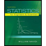
Statistics for Engineers and Scientists
4th Edition
ISBN: 9780073401331
Author: William Navidi Prof.
Publisher: McGraw-Hill Education
expand_more
expand_more
format_list_bulleted
Concept explainers
Textbook Question
Chapter 7.2, Problem 1E
Each month for several months, the average temperature in °C (x) and the number of pounds of steam (y) consumed by a certain chemical plant were measured. The least-squares line computed from the resulting data is y = 245.82 + 1.13x.
- a. Predict the number of pounds of steam consumed in a month where the average temperature is 65°C.
- b. If two months differ in their average temperatures by 5°C, by how much do you predict the number of pounds of steam consumed to differ?
Expert Solution & Answer
Want to see the full answer?
Check out a sample textbook solution
Students have asked these similar questions
1. Let 2 (a, b, c)} be the sample space.
(a) Write down the power set of 2.
(b) Construct a σ-field containing A = {a, b} and B = {b, c}.
(c) Show that F= {0, 2, {a, b}, {b, c}, {b}} is not a σ-field. Add some elements
to make it a σ-field..
13. Let (, F, P) be a probability space and X a function from 2 to R. Explain when
X is a random variable.
24. A factory produces items from two machines: Machine A and Machine B. Machine
A produces 60% of the total items, while Machine B produces 40%. The probability
that an item produced by Machine A is defective is P(DIA)=0.03. The probability
that an item produced by Machine B is defective is P(D|B)=0.05.
(a) What is the probability that a randomly selected product be defective, P(D)?
(b) If a randomly selected item from the production line is defective, calculate the
probability that it was produced by Machine A, P(A|D).
Chapter 7 Solutions
Statistics for Engineers and Scientists
Ch. 7.1 - Compute the correlation coefficient for the...Ch. 7.1 - For each of the following data sets, explain why...Ch. 7.1 - For each of the following scatterplots, state...Ch. 7.1 - True or false, and explain briefly: a. If the...Ch. 7.1 - In a study of ground motion caused by earthquakes,...Ch. 7.1 - A chemical engineer is studying the effect of...Ch. 7.1 - Another chemical engineer is studying the same...Ch. 7.1 - Tire pressure (in kPa) was measured for the right...Ch. 7.1 - Prob. 10ECh. 7.1 - The article Drift in Posturography Systems...
Ch. 7.1 - Prob. 12ECh. 7.1 - Prob. 13ECh. 7.1 - A scatterplot contains four points: (2, 2), (1,...Ch. 7.2 - Each month for several months, the average...Ch. 7.2 - In a study of the relationship between the Brinell...Ch. 7.2 - A least-squares line is fit to a set of points. If...Ch. 7.2 - Prob. 4ECh. 7.2 - In Galtons height data (Figure 7.1, in Section...Ch. 7.2 - In a study relating the degree of warping, in mm....Ch. 7.2 - Moisture content in percent by volume (x) and...Ch. 7.2 - The following table presents shear strengths (in...Ch. 7.2 - Structural engineers use wireless sensor networks...Ch. 7.2 - The article Effect of Environmental Factors on...Ch. 7.2 - An agricultural scientist planted alfalfa on...Ch. 7.2 - Curing times in days (x) and compressive strengths...Ch. 7.2 - Prob. 13ECh. 7.2 - An engineer wants to predict the value for y when...Ch. 7.2 - A simple random sample of 100 men aged 2534...Ch. 7.2 - Prob. 16ECh. 7.3 - A chemical reaction is run 12 times, and the...Ch. 7.3 - Structural engineers use wireless sensor networks...Ch. 7.3 - Prob. 3ECh. 7.3 - Prob. 4ECh. 7.3 - Prob. 5ECh. 7.3 - Prob. 6ECh. 7.3 - The coefficient of absorption (COA) for a clay...Ch. 7.3 - Prob. 8ECh. 7.3 - Prob. 9ECh. 7.3 - Three engineers are independently estimating the...Ch. 7.3 - In the skin permeability example (Example 7.17)...Ch. 7.3 - Prob. 12ECh. 7.3 - In a study of copper bars, the relationship...Ch. 7.3 - Prob. 14ECh. 7.3 - In the following MINITAB output, some of the...Ch. 7.3 - Prob. 16ECh. 7.3 - In order to increase the production of gas wells,...Ch. 7.4 - The following output (from MINITAB) is for the...Ch. 7.4 - The processing of raw coal involves washing, in...Ch. 7.4 - To determine the effect of temperature on the...Ch. 7.4 - The depth of wetting of a soil is the depth to...Ch. 7.4 - Good forecasting and control of preconstruction...Ch. 7.4 - The article Drift in Posturography Systems...Ch. 7.4 - Prob. 7ECh. 7.4 - Prob. 8ECh. 7.4 - A windmill is used to generate direct current....Ch. 7.4 - Two radon detectors were placed in different...Ch. 7.4 - Prob. 11ECh. 7.4 - The article The Selection of Yeast Strains for the...Ch. 7.4 - Prob. 13ECh. 7.4 - The article Characteristics and Trends of River...Ch. 7.4 - Prob. 15ECh. 7.4 - The article Mechanistic-Empirical Design of...Ch. 7.4 - An engineer wants to determine the spring constant...Ch. 7 - The BeerLambert law relates the absorbance A of a...Ch. 7 - Prob. 2SECh. 7 - Prob. 3SECh. 7 - Refer to Exercise 3. a. Plot the residuals versus...Ch. 7 - Prob. 5SECh. 7 - The article Experimental Measurement of Radiative...Ch. 7 - Prob. 7SECh. 7 - Prob. 8SECh. 7 - Prob. 9SECh. 7 - Prob. 10SECh. 7 - The article Estimating Population Abundance in...Ch. 7 - A materials scientist is experimenting with a new...Ch. 7 - Monitoring the yield of a particular chemical...Ch. 7 - Prob. 14SECh. 7 - Refer to Exercise 14. Someone wants to compute a...Ch. 7 - Prob. 16SECh. 7 - Prob. 17SECh. 7 - Prob. 18SECh. 7 - Prob. 19SECh. 7 - Use Equation (7.34) (page 545) to show that 1=1.Ch. 7 - Use Equation (7.35) (page 545) to show that 0=0.Ch. 7 - Prob. 22SECh. 7 - Use Equation (7.35) (page 545) to derive the...
Additional Math Textbook Solutions
Find more solutions based on key concepts
The largest polynomial that divides evenly into a list of polynomials is called the _______.
Elementary & Intermediate Algebra
Check Your Understanding
Reading Check Complete each sentence using > or < for □.
RC1. 3 dm □ 3 dam
Basic College Mathematics
Empirical versus Theoretical A Monopoly player claims that the probability of getting a 4 when rolling a six-si...
Introductory Statistics
Evaluate the integrals in Exercises 1–46.
1.
University Calculus: Early Transcendentals (4th Edition)
Provide an example of a qualitative variable and an example of a quantitative variable.
Elementary Statistics ( 3rd International Edition ) Isbn:9781260092561
NOTE: Write your answers using interval notation when appropriate.
CHECKING ANALYTIC SKILLS Fill in each blank ...
Graphical Approach To College Algebra
Knowledge Booster
Learn more about
Need a deep-dive on the concept behind this application? Look no further. Learn more about this topic, statistics and related others by exploring similar questions and additional content below.Similar questions
- (b) In various places in this module, data on the silver content of coins minted in the reign of the twelfth-century Byzantine king Manuel I Comnenus have been considered. The full dataset is in the Minitab file coins.mwx. The dataset includes, among others, the values of the silver content of nine coins from the first coinage (variable Coin1) and seven from the fourth coinage (variable Coin4) which was produced a number of years later. (For the purposes of this question, you can ignore the variables Coin2 and Coin3.) In particular, in Activity 8 and Exercise 2 of Computer Book B, it was argued that the silver contents in both the first and the fourth coinages can be assumed to be normally distributed. The question of interest is whether there were differences in the silver content of coins minted early and late in Manuel’s reign. You are about to investigate this question using a two-sample t-interval. (i) Using Minitab, find either the sample standard deviations of the two variables…arrow_forwardHomework Let X1, X2, Xn be a random sample from f(x;0) where f(x; 0) = (-), 0 < x < ∞,0 € R Using Basu's theorem, show that Y = min{X} and Z =Σ(XY) are indep. -arrow_forwardHomework Let X1, X2, Xn be a random sample from f(x; 0) where f(x; 0) = e−(2-0), 0 < x < ∞,0 € R Using Basu's theorem, show that Y = min{X} and Z =Σ(XY) are indep.arrow_forward
- An Arts group holds a raffle. Each raffle ticket costs $2 and the raffle consists of 2500 tickets. The prize is a vacation worth $3,000. a. Determine your expected value if you buy one ticket. b. Determine your expected value if you buy five tickets. How much will the Arts group gain or lose if they sell all the tickets?arrow_forwardPlease show as much work as possible to clearly show the steps you used to find each solution. If you plan to use a calculator, please be sure to clearly indicate your strategy. Consider the following game. It costs $3 each time you roll a six-sided number cube. If you roll a 6 you win $15. If you roll any other number, you receive nothing. a) Find the expected value of the game. b) If you play this game many times, will you expect to gain or lose money?arrow_forward= 12:02 WeBWorK / 2024 Fall Rafeek MTH23 D02 / 9.2 Testing the Mean mu / 3 38 WEBWORK Previous Problem Problem List Next Problem 9.2 Testing the Mean mu: Problem 3 (1 point) Test the claim that the population of sophomore college students has a mean grade point average greater than 2.2. Sample statistics include n = 71, x = 2.44, and s = 0.9. Use a significance level of a = 0.01. The test statistic is The P-Value is between : The final conclusion is < P-value < A. There is sufficient evidence to support the claim that the mean grade point average is greater than 2.2. ○ B. There is not sufficient evidence to support the claim that the mean grade point average is greater than 2.2. Note: You can earn partial credit on this problem. Note: You are in the Reduced Scoring Period. All work counts for 50% of the original. Preview My Answers Submit Answers You have attempted this problem 0 times. You have unlimited attempts remaining. . Oli wwm01.bcc.cuny.eduarrow_forward
- There are four white, fourteen blue and five green marbles in a bag. A marble is selected from the bag without looking. Find the odds of the following: The odds against selecting a green marble. The odds in favour of not selecting a green marble The odds in favor of the marble selected being either a white or a blue marble. What is true about the above odds? Explainarrow_forwardPlease show as much work as possible to clearly show the steps you used to find each solution. If you plan to use a calculator, please be sure to clearly indicate your strategy. 1. The probability of a soccer game in a particular league going into overtime is 0.125. Find the following: a. The odds in favour of a game going into overtime. b. The odds in favour of a game not going into overtime. c. If the teams in the league play 100 games in a season, about how many games would you expect to go into overtime?arrow_forwardexplain the importance of the Hypothesis test in a business setting, and give an example of a situation where it is helpful in business decision making.arrow_forward
- A college wants to estimate what students typically spend on textbooks. A report fromthe college bookstore observes that textbooks range in price from $22 to $186. Toobtain a 95% confidence level for a confidence interval estimate to plus or minus $10,how many students should the college survey? (We may estimate the populationstandard deviation as (range) ÷ 4.)arrow_forwardIn a study of how students give directions, forty volunteers were given the task ofexplaining to another person how to reach a destination. Researchers measured thefollowing five aspects of the subjects’ direction-giving behavior:• whether a map was available or if directions were given from memory without a map,• the gender of the direction-giver,• the distances given as part of the directions,• the number of times directions such as “north” or “left” were used,• the frequency of errors in directions. Identify each of the variables in this study, and whether each is quantitative orqualitative. For each quantitative variable, state whether it is discrete or continuous. Was this an observational study or an experimental study? Explain your answer.arrow_forwardexplain the difference between the confident interval and the confident level. provide an example to show how to correctly interpret a confidence interval.arrow_forward
arrow_back_ios
SEE MORE QUESTIONS
arrow_forward_ios
Recommended textbooks for you
- Algebra & Trigonometry with Analytic GeometryAlgebraISBN:9781133382119Author:SwokowskiPublisher:Cengage
 Functions and Change: A Modeling Approach to Coll...AlgebraISBN:9781337111348Author:Bruce Crauder, Benny Evans, Alan NoellPublisher:Cengage Learning
 Glencoe Algebra 1, Student Edition, 9780079039897...AlgebraISBN:9780079039897Author:CarterPublisher:McGraw Hill
 Algebra: Structure And Method, Book 1AlgebraISBN:9780395977224Author:Richard G. Brown, Mary P. Dolciani, Robert H. Sorgenfrey, William L. ColePublisher:McDougal Littell

Algebra & Trigonometry with Analytic Geometry
Algebra
ISBN:9781133382119
Author:Swokowski
Publisher:Cengage

Functions and Change: A Modeling Approach to Coll...
Algebra
ISBN:9781337111348
Author:Bruce Crauder, Benny Evans, Alan Noell
Publisher:Cengage Learning

Glencoe Algebra 1, Student Edition, 9780079039897...
Algebra
ISBN:9780079039897
Author:Carter
Publisher:McGraw Hill


Algebra: Structure And Method, Book 1
Algebra
ISBN:9780395977224
Author:Richard G. Brown, Mary P. Dolciani, Robert H. Sorgenfrey, William L. Cole
Publisher:McDougal Littell

Use of ALGEBRA in REAL LIFE; Author: Fast and Easy Maths !;https://www.youtube.com/watch?v=9_PbWFpvkDc;License: Standard YouTube License, CC-BY
Compound Interest Formula Explained, Investment, Monthly & Continuously, Word Problems, Algebra; Author: The Organic Chemistry Tutor;https://www.youtube.com/watch?v=P182Abv3fOk;License: Standard YouTube License, CC-BY
Applications of Algebra (Digit, Age, Work, Clock, Mixture and Rate Problems); Author: EngineerProf PH;https://www.youtube.com/watch?v=Y8aJ_wYCS2g;License: Standard YouTube License, CC-BY