
Videos
An accurate assessment of oxygen consumption provides important information for determining energy expenditure requirements for physically demanding tasks. The paper “Oxygen Consumption During Fire Suppression: Error of Heart Rate Estimation” (Ergonomics [1991]: 1469–1474) reported on a study in which x = Oxygen consumption (in milliliters per kilogram per minute) during a treadmill test was determined for a sample of 10 firefighters. Then y = Oxygen consumption at a comparable heart rate was measured for each of the 10 individuals while they performed a fire-suppression simulation. This resulted in the following data and

- a. Does the scatterplot suggest an approximate linear relationship?
- b. The investigators fit a least-squares line. The resulting Minitab output is given in the following:
The regression equation is firecon = 211. 4 + 1. 09 treadcon
Predict fire-simulation consumption when treadmill consumption is 40.
- c. How effectively does a straight line summarize the relationship?
- d. Delete the first observation, (51.3, 49.3), and calculate the new equation of the least-squares line and the value of r2. What do you conclude? (Hint: For the original data, Σx = 388.8, Σy = 310 .3, Σx2 = 15,338.54, Σxy = 12,306.58, and Σy2 = 10,072.41.)
a.
Discuss whether the scatterplot indicates an approximate linear relationship.
Answer to Problem 78CR
No, the scatterplot does not indicate an approximate linear relationship.
Explanation of Solution
The data relates the oxygen consumption (milliliters per kilogram per minute) of 10 firefighters during a fire-suppression simulation, y to that during a treadmill test, x. The scatterplot between the two variables is given.
Denote the estimated response variable as ˆy.
A careful inspection of the given scatterplot shows that the points do not fall on a straight line. Rather, the points are scattered almost in a random manner, without showing any pattern in particular. However, there is one extreme point, which is far away from the remaining points. This extreme point appears to provide an impression that there might be a linear relationship between the two variables. Once this point is ignored, it is clear that no such relationship can be determined.
Thus, the scatterplot does not indicate an approximate linear relationship.
b.
Predict the fire-simulation oxygen consumption, if the treadmill oxygen consumption is 40.
Answer to Problem 78CR
The fire-simulation oxygen consumption, when the treadmill oxygen consumption is 40 is 32.254 milliliters per kilogram per minute.
Explanation of Solution
Calculation:
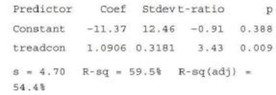
The MINITAB output for the fitting of a least-squares regression line to the given data is given.
In the given output, the column of “Coef” gives the coefficients corresponding to the variables given in the column of “Predictor”. The term “Constant” under the column of ‘Predictor’ gives the intercept of the equation; the term “treadcon” denotes the oxygen consumption of during the treadmill test, x.
Using the values in the output, the equation of the least-squares regression line is ˆy=−11.37+1.0906x.
For a treadmill oxygen consumption of 40 milliliters per kilogram per minute, x=40. Substitute this value in the above least-squares equation to predict the response variable:
ˆy=−11.37+1.0906x=−11.37+(1.0906×40)=−11.37+43.624=32.254.
Thus, the fire-simulation oxygen consumption, when the treadmill oxygen consumption is 40 is 32.254 milliliters per kilogram per minute.
c.
Explain the effectivity of the straight line to summarize the relationship between the variables.
Explanation of Solution
In the given output, the value of r2 is reported as R-sq=59.5%.
Now, r2 is the percentage of variability in the response variable that can be explained by the regression model involving the given predictor variable.
Thus, it can be interpreted that the oxygen consumption during the treadmill test can predict about 59.5% of the variability in the oxygen consumption during the fire-suppression simulation.
This suggests that the straight line is moderately effective in summarizing the relationship between the variables.
d.
Find the equation of the least-squares line and the value of r2, after deleting the first observation, (51.3, 49.3).
Answer to Problem 78CR
The equation of the least-squares line after deleting the first observation, (51.3, 49.3) is ˆy=36.4175−0.1978x_.
The value of r2 after deleting the first observation, (51.3, 49.3) is 0.02.
Explanation of Solution
Calculation:
It is given that, for the original data set, ∑x=388.8, ∑y=310.3, ∑x2=15,338.54, ∑xy=12,306.58 and ∑y2=10,072.41. The first observation, (51.3, 49.3) is deleted. Thus, the new data set contains n=9 observations.
For the first observation, x=51.3, y=49.3. If this observation is deleted, the values of ∑x, ∑y, ∑x2, ∑xy and ∑y2 change as follows:
∑x=388.8−51.3=337.5.
∑y=310.3−49.3=261.
∑x2=15,338.54−(51.3)2=15,338.54−2,631.69=12,706.85.
∑xy=12,306.58−(51.3)⋅(49.3)=12,306.58−2,529.09=9,777.49.
∑y2=10,072.41−(49.3)2=10,072.41−2,430.49=7,641.92.
Now, the lest-squares regression line is of the form: ˆy=a+bx, where the intercept, a=ˉy−bˉx and the slope, b=∑xy−(∑x)(∑y)n∑x2−(∑x)2n, with ˉy denoting the mean of the response variable, y.
Using this formula and the values obtained above, b and a are respectively obtained as follows:
b=∑xy−(∑x)(∑y)n∑x2−(∑x)2n=9,777.49−(337.5)(261)912,706.85−(337.5)29=9,777.49−9,787.512,706.85−12,656.25=−10.0150.6≈−0.1978.
Now,
ˉx=1n∑x=337.59=37.5.
ˉy=1n∑y=2619=29.
Thus,
a=ˉy−bˉx=29−(−0.1978)⋅(37.5)=29+7.4175=36.4175.
Using the values of a and b obtained above, the equation of the least-squares line after deleting the first observation, (51.3, 49.3) is ˆy=36.4175−0.1978x_.
Now, it is known that the slope for the least-squares regression of y on x, that is, b can be given by the formula: b=rsysx, where sx and sy are respectively the standard deviations of x and y. As a result, r=bsxsy.
Now, it can be shown that:
sx=√∑(x−ˉx)2n−1=√∑x2−∑xnn−1.
Similarly,
sy=√∑(y−ˉy)2n−1=√∑y2−∑ynn−1.
Thus,
r=bsxsy=b√∑x2−(∑x)nn−1√∑y2−(∑y)nn−1=b√∑x2−(∑x)2n√∑y2−(∑y)2n.
Using the values obtained above, the value of r can be calculated as follows:
r=b√∑x2−(∑x)2n√∑y2−(∑y)2n=(−0.1978)√50.6√7,641.92−(261)29=(−0.1978)√50.6√7,641.92−7,569=(−0.1978)√50.6√92.92≈−0.146.
It is known that r2 is simply the square of r. Thus,
r2=(−0.146)2≈0.02.
Hence, the value of r2 after deleting the first observation, (51.3, 49.3) is 0.02.
Now, r2 multiplied by 100, gives the percentage of variability in the response variable that can be explained by the regression model involving the given predictor variable.
Now,
100r2=100×0.02=2%.
Thus, it can be interpreted that the oxygen consumption during the treadmill test can predict about 2% of the variability in the oxygen consumption during the fire-suppression simulation, which is a very low percentage.
Thus, the model 9is not a very good fit for the data.
Want to see more full solutions like this?
Chapter 5 Solutions
Introduction To Statistics And Data Analysis
Additional Math Textbook Solutions
Calculus: Early Transcendentals (2nd Edition)
Precalculus
APPLIED STAT.IN BUS.+ECONOMICS
Elementary Statistics: Picturing the World (7th Edition)
College Algebra (Collegiate Math)


- Exercise 6-6 (Algo) (LO6-3) The director of admissions at Kinzua University in Nova Scotia estimated the distribution of student admissions for the fall semester on the basis of past experience. Admissions Probability 1,100 0.5 1,400 0.4 1,300 0.1 Click here for the Excel Data File Required: What is the expected number of admissions for the fall semester? Compute the variance and the standard deviation of the number of admissions. Note: Round your standard deviation to 2 decimal places.arrow_forward1. Find the mean of the x-values (x-bar) and the mean of the y-values (y-bar) and write/label each here: 2. Label the second row in the table using proper notation; then, complete the table. In the fifth and sixth columns, show the 'products' of what you're multiplying, as well as the answers. X y x minus x-bar y minus y-bar (x minus x-bar)(y minus y-bar) (x minus x-bar)^2 xy 16 20 34 4-2 5 2 3. Write the sums that represents Sxx and Sxy in the table, at the bottom of their respective columns. 4. Find the slope of the Regression line: bi = (simplify your answer) 5. Find the y-intercept of the Regression line, and then write the equation of the Regression line. Show your work. Then, BOX your final answer. Express your line as "y-hat equals...arrow_forwardApply STATA commands & submit the output for each question only when indicated below i. Generate the log of birthweight and family income of children. Name these new variables Ibwght & Ifaminc. Include the output of this code. ii. Apply the command sum with the detail option to the variable faminc. Note: you should find the 25th percentile value, the 50th percentile and the 75th percentile value of faminc from the output - you will need it to answer the next question Include the output of this code. iii. iv. Use the output from part ii of this question to Generate a variable called "high_faminc" that takes a value 1 if faminc is less than or equal to the 25th percentile, it takes the value 2 if faminc is greater than 25th percentile but less than or equal to the 50th percentile, it takes the value 3 if faminc is greater than 50th percentile but less than or equal to the 75th percentile, it takes the value 4 if faminc is greater than the 75th percentile. Include the outcome of this code…arrow_forward
- solve this on paperarrow_forwardApply STATA commands & submit the output for each question only when indicated below i. Apply the command egen to create a variable called "wyd" which is the rowtotal function on variables bwght & faminc. ii. Apply the list command for the first 10 observations to show that the code in part i worked. Include the outcome of this code iii. Apply the egen command to create a new variable called "bwghtsum" using the sum function on variable bwght by the variable high_faminc (Note: need to apply the bysort' statement) iv. Apply the "by high_faminc" statement to find the V. descriptive statistics of bwght and bwghtsum Include the output of this code. Why is there a difference between the standard deviations of bwght and bwghtsum from part iv of this question?arrow_forwardAccording to a health information website, the distribution of adults’ diastolic blood pressure (in millimeters of mercury, mmHg) can be modeled by a normal distribution with mean 70 mmHg and standard deviation 20 mmHg. b. Above what diastolic pressure would classify someone in the highest 1% of blood pressures? Show all calculations used.arrow_forward
- Write STATA codes which will generate the outcomes in the questions & submit the output for each question only when indicated below i. ii. iii. iv. V. Write a code which will allow STATA to go to your favorite folder to access your files. Load the birthweight1.dta dataset from your favorite folder and save it under a different filename to protect data integrity. Call the new dataset babywt.dta (make sure to use the replace option). Verify that it contains 2,998 observations and 8 variables. Include the output of this code. Are there missing observations for variable(s) for the variables called bwght, faminc, cigs? How would you know? (You may use more than one code to show your answer(s)) Include the output of your code (s). Write the definitions of these variables: bwght, faminc, male, white, motheduc,cigs; which of these variables are categorical? [Hint: use the labels of the variables & the browse command] Who is this dataset about? Who can use this dataset to answer what kind of…arrow_forwardApply STATA commands & submit the output for each question only when indicated below İ. ii. iii. iv. V. Apply the command summarize on variables bwght and faminc. What is the average birthweight of babies and family income of the respondents? Include the output of this code. Apply the tab command on the variable called male. How many of the babies and what share of babies are male? Include the output of this code. Find the summary statistics (i.e. use the sum command) of the variables bwght and faminc if the babies are white. Include the output of this code. Find the summary statistics (i.e. use the sum command) of the variables bwght and faminc if the babies are male but not white. Include the output of this code. Using your answers to previous subparts of this question: What is the difference between the average birthweight of a baby who is male and a baby who is male but not white? What can you say anything about the difference in family income of the babies that are male and male…arrow_forwardA public health researcher is studying the impacts of nudge marketing techniques on shoppers vegetablesarrow_forward
- The director of admissions at Kinzua University in Nova Scotia estimated the distribution of student admissions for the fall semester on the basis of past experience. Admissions Probability 1,100 0.5 1,400 0.4 1,300 0.1 Click here for the Excel Data File Required: What is the expected number of admissions for the fall semester? Compute the variance and the standard deviation of the number of admissions. Note: Round your standard deviation to 2 decimal places.arrow_forwardA pollster randomly selected four of 10 available people. Required: How many different groups of 4 are possible? What is the probability that a person is a member of a group? Note: Round your answer to 3 decimal places.arrow_forwardWind Mountain is an archaeological study area located in southwestern New Mexico. Potsherds are broken pieces of prehistoric Native American clay vessels. One type of painted ceramic vessel is called Mimbres classic black-on-white. At three different sites the number of such sherds was counted in local dwelling excavations. Test given. Site I Site II Site III 63 19 60 43 34 21 23 49 51 48 11 15 16 46 26 20 31 Find .arrow_forward
 Glencoe Algebra 1, Student Edition, 9780079039897...AlgebraISBN:9780079039897Author:CarterPublisher:McGraw Hill