
Concept explainers
Videos
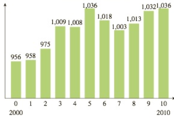
College Basketball: Women The following chart shows the number of NCAA women’s college basketball teams in the United States during the period 2000–2010:43
Men’s basketball teams
Year (t)
a. On average, how fast was the number of women’s college basketball teams growing over the 4-year period beginning in 2004?
b. By inspecting the graph, find the 3-year period over which the average rate of change was largest.
Want to see the full answer?
Check out a sample textbook solution
Chapter 3 Solutions
Applied Calculus
Additional Math Textbook Solutions
Finite Mathematics and Calculus with Applications (10th Edition)
Calculus, Single Variable: Early Transcendentals (3rd Edition)
Calculus: Single And Multivariable
Advanced Mathematical Concepts: Precalculus with Applications, Student Edition
University Calculus: Early Transcendentals (4th Edition)
Single Variable Calculus: Early Transcendentals (2nd Edition) - Standalone book


- Using the data in Table 6–11, calculate a 3-month moving average forecast for month 12.arrow_forwardThe following chart shows "living wage" jobs in Tucson per 1000 working age adults over a 5 year period. Year 2007 2008 2009 2010 2011 Jobs 675 720 760 795 820 What is the average rate of change in the number of living wage jobs from 2007 to 2009? Jobs/Year What is the average rate of change in the number of living wage jobs from 2009 to 2011? Jobs/Yeararrow_forwardQ1. The table provided gives data on indexes of output per hour (X) and real compensation per hour (Y) for the business and nonfarm business sectors of the U.S. economy for 1960–2005. The base year of the indexes is 1992 = 100 and the indexes are seasonally adjusted. a. Plot Y against X for the two sectors separately. b. What is the economic theory behind the relationship between the two variables? Does the scattergram support the theory? c. Estimate the OLS regression of Y on X. Note: on the table ( 1. Output refers to real gross domestic product in the sector. 2. Wages and salaries of employees plus employers’ contributions for social insurance and private benefit plans. 3. Hourly compensation divided by the consumer price index for all urban consumers for recent quarters.) Thank you!arrow_forward
- The Internal Revenue Service Restructuring and Reform Act (RRA) was signed into law by President Bill Clinton in 1998. A major objective of the RRA was to promote electronic filing of tax returns. The data in the table that follows show the percentage of individual income tax returns filed electronically for filing years 2000–2008. Since the percentage P of returns filed electronically depends on the filing year y and each input corresponds to exactly one output, the percentage of returns filed electronically is a function of the filing year;so P(y) represents the percentage of returns filed electronically for filing year y. (a) Find the average rate of change of the percentage of e-filed returns from 2000 to 2002. (b) Find the average rate of change of the percentage of e-filed returns from 2004 to 2006. (c) Find the average rate of change of the percentage of e-filed returns from 2006 to 2008. (d) What is happening to the average rate of change as time passes?arrow_forwardThe figure below shows timber production in particular months from 2000 to 2005. Which of the following months of the year seems to have the lowest timber production? (a) January (b) April (c) July (d) Octoberarrow_forwardThe body mass index (BMI) of a person is the person’s weight divided by the square of his or her height. It is an indirect measure of the person’s body fat and an indicator of obesity. Results from surveys conducted by the Centers for Disease Control and Prevention (CDC) showed that the estimated mean BMI for US adults increased from 25.0 in the 1960–1962 period to 28.1 in the 1999–2002 period. [Source: Ogden, C., et al. (2004). Mean body weight, height, and body mass index, United States 1960–2002. Suppose you are a health researcher. You conduct a hypothesis test to determine whether the mean BMI of US adults in the current year is greater than the mean BMI of US adults in 2000. Assume that the mean BMI of US adults in 2000 was 28.1 (the population mean). You obtain a sample of BMI measurements of 1,034 US adults, which yields a sample mean of M = 28.9. Let μ denote the mean BMI of US adults in the current year. Please Formulate the null and alternative hypothesesarrow_forward
