
Videos
The dynamics of a forced spring-mass-damper system can be represented by the following second-order ODE:
where
(a)
To calculate: The displacement and velocity as a function of time for linear system where
Answer to Problem 49P
Solution:
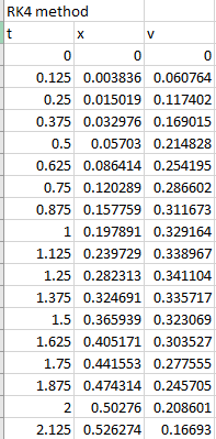
The first few solutions for displacement and velocity as a function of time for liner system is,
| t | x | v |
| 0 | 0 | 0 |
| 0.125 | 0.003836 | 0.060764 |
| 0.25 | 0.015019 | 0.117402 |
| 0.375 | 0.032976 | 0.169015 |
| 0.5 | 0.05703 | 0.214828 |
| 0.625 | 0.086414 | 0.254195 |
| 0.75 | 0.120289 | 0.286602 |
| 0.875 | 0.157759 | 0.311673 |
| 1 | 0.197891 | 0.329164 |
| 1.125 | 0.239729 | 0.338967 |
| 1.25 | 0.282313 | 0.341104 |
| 1.375 | 0.324691 | 0.335717 |
| 1.5 | 0.365939 | 0.323069 |
| 1.625 | 0.405171 | 0.303527 |
| 1.75 | 0.441553 | 0.277555 |
| 1.875 | 0.474314 | 0.245705 |
| 2 | 0.50276 | 0.208601 |
| 2.125 | 0.526274 | 0.16693 |
| 2.25 | 0.544332 | 0.121428 |
| 2.375 | 0.556503 | 0.072863 |
| 2.5 | 0.562454 | 0.02203 |
| 2.625 | 0.56195 | -0.03027 |
| 2.75 | 0.554859 | -0.08324 |
| 2.875 | 0.541146 | -0.13608 |
| 3 | 0.520874 | -0.18805 |
| 3.125 | 0.494199 | -0.23842 |
| 3.25 | 0.461364 | -0.28651 |
| 3.375 | 0.422694 | -0.33168 |
| 3.5 | 0.378588 | -0.37339 |
| 3.625 | 0.329513 | -0.41112 |
| 3.75 | 0.275993 | -0.44444 |
| 3.875 | 0.218601 | -0.47301 |
| 4 | 0.157952 | -0.49653 |
| 4.125 | 0.094688 | -0.5148 |
| 4.25 | 0.029475 | -0.52771 |
| 4.375 | -0.03701 | -0.53518 |
| 4.5 | -0.1041 | -0.53725 |
| 4.625 | -0.1711 | -0.53399 |
| 4.75 | -0.23738 | -0.52558 |
| 4.875 | -0.30229 | -0.51221 |
| 5 | -0.36524 | -0.49416 |
Explanation of Solution
Given Information:
The dynamic of a forced spring-mass-damper system is given as,
The values,
The initial condition,
Formula used:
The fourth-order RK method for
Where,
Calculation:
Consider the dynamic of a forced spring-mass-damper system,
As
Divide both the sides of above equation by m,
Now, substitute the values
For linear, substitute
Use VBA code for RK4 method as below to solve for x and v,
Code:
Output:
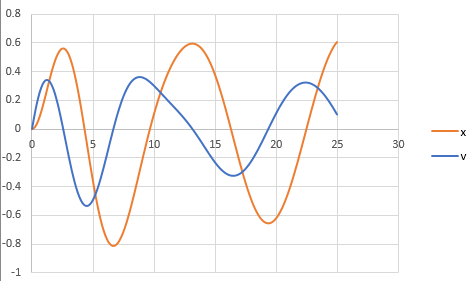
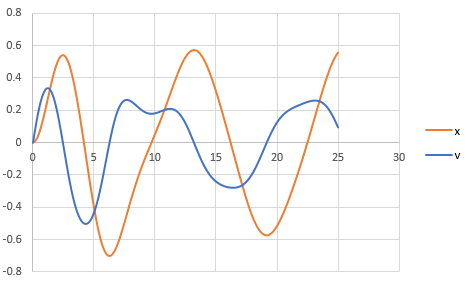
To draw the graph of the above results, follow the steps in excel sheet as given below,
Step 1: Select the cell from A4 to A205 and cell B4 to B205. Then, go to the Insert and select the scatter with smooth lines from the chart.
Step 2: Select the cell from A4 to A205 and cell C4 to C205. Then, go to the Insert and select the scatter with smooth lines from the chart.
Step 3: Select one of the graphs and paste it on another graph to merge the graphs.
The graph obtained is,
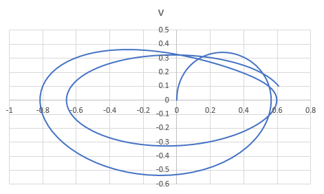
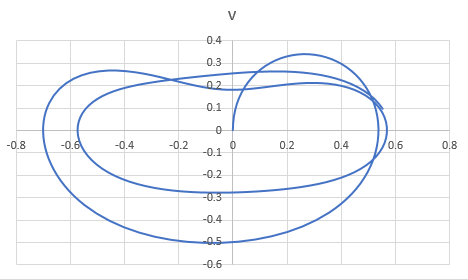
And, to draw the phase plane plot follow the steps as below,
Step 4: Select the column B and column C. Then, go to the Insert and select the scatter with smooth lines from the chart.
The graph obtained is,
(b)
To calculate: The displacement and velocity as a function of time for non-linear system where
Answer to Problem 49P
Solution:
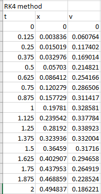
| t | x | v |
| 0 | 0 | 0 |
| 0.125 | 0.003836 | 0.060764 |
| 0.25 | 0.015019 | 0.117402 |
| 0.375 | 0.032976 | 0.169014 |
| 0.5 | 0.05703 | 0.214821 |
| 0.625 | 0.086412 | 0.254166 |
| 0.75 | 0.120279 | 0.286506 |
| 0.875 | 0.157729 | 0.311417 |
| 1 | 0.19781 | 0.328581 |
| 1.125 | 0.239542 | 0.337784 |
| 1.25 | 0.28192 | 0.338923 |
| 1.375 | 0.323936 | 0.332004 |
| 1.5 | 0.36459 | 0.31716 |
| 1.625 | 0.402907 | 0.294658 |
| 1.75 | 0.437953 | 0.264919 |
| 1.875 | 0.468859 | 0.228524 |
| 2 | 0.494837 | 0.186221 |
| 2.125 | 0.515205 | 0.138911 |
| 2.25 | 0.5294 | 0.087637 |
| 2.375 | 0.536996 | 0.033543 |
| 2.5 | 0.537718 | -0.02217 |
| 2.625 | 0.531437 | -0.07829 |
| 2.75 | 0.518177 | -0.13366 |
| 2.875 | 0.498099 | -0.18721 |
| 3 | 0.47149 | -0.23801 |
| 3.125 | 0.438743 | -0.28531 |
| 3.25 | 0.400333 | -0.32852 |
| 3.375 | 0.3568 | -0.36723 |
| 3.5 | 0.308725 | -0.40117 |
| 3.625 | 0.256712 | -0.43023 |
| 3.75 | 0.201374 | -0.45436 |
| 3.875 | 0.143325 | -0.47361 |
| 4 | 0.083172 | -0.48804 |
| 4.125 | 0.021513 | -0.49771 |
| 4.25 | -0.04106 | -0.50268 |
| 4.375 | -0.10396 | -0.50296 |
| 4.5 | -0.1666 | -0.49854 |
| 4.625 | -0.2284 | -0.48938 |
| 4.75 | -0.28875 | -0.47544 |
| 4.875 | -0.34705 | -0.45667 |
| 5 | -0.40271 | -0.43306 |
Explanation of Solution
Given Information:
The dynamic of a forced spring-mass-damper system is given as,
The values,
And,
The initial condition,
Formula used:
The fourth-order RK method for
Where,
Calculation:
Consider the dynamic of a forced spring-mass-damper system,
As
Divide both the sides of above equation by m,
Now, substitute the values
For linear, substitute
Use VBA code for RK4 method as below to solve for x and v,
Code:
Output:
Few data are shown below,
To draw the graph of the above results, follow the steps in excel sheet as given below,
Step 1: Select the cell from A4 to A205 and cell B4 to B205. Then, go to the Insert and select the scatter with smooth lines from the chart.
Step 2: Select the cell from A4 to A205 and cell C4 to C205. Then, go to the Insert and select the scatter with smooth lines from the chart.
Step 3: Select one of the graphs and paste it on another graph to merge the graphs.
The graph obtained is,
And, to draw the phase plane plot follow the steps as below,
Step 4: Select the column B and column C. Then, go to the Insert and select the scatter with smooth lines from the chart.
The graph obtained is,
Want to see more full solutions like this?
Chapter 28 Solutions
EBK NUMERICAL METHODS FOR ENGINEERS


- Harmonic oscillators. One of the simplest yet most important second-order, linear, constant- coefficient differential equations is the equation for a harmonic oscilator. This equation models the motion of a mass attached to a spring. The spring is attached to a vertical wall and the mass is allowed to slide along a horizontal track. We let z denote the displacement of the mass from its natural resting place (with x > 0 if the spring is stretched and x 0 is the damping constant, and k> 0 is the spring constant. Newton's law states that the force acting on the oscillator is equal to mass times acceleration. Therefore the differential equation for the damped harmonic oscillator is mx" + bx' + kr = 0. (1) k Lui Assume the mass m = 1. (a) Transform Equation (1) into a system of first-order equations. (b) For which values of k, b does this system have complex eigenvalues? Repeated eigenvalues? Real and distinct eigenvalues? (c) Find the general solution of this system in each case. (d)…arrow_forward= = Problem #2 - Modeling, Mass-Spring System Two masses are connected by springs in series as shown in Figure 1 below where k₁ 20 N/m, k₂ = 10 N/m, m₁ 10 kg, and m₂ = 5 kg. Solve the system of ODEs in matrix form using the determinant to obtain the characteristic equation (it will make sense to substitute > for w² when you get to your characteristic equation). Determine the eigenvalues (frequencies) and eigenvectors (modes) of oscillation. Assume that no damping is present and that the masses slide without friction. On your diagram, sketch the modes of oscillation (think of how the masses could oscillate with respect to each other). What determines which mode or combination of modes that the masses oscillate at? i.) ii.) iii.) iv.) v.) vi.) vii.) Sketch the system and include a free body diagram. Use a conservation equation to develop your differential equation model (you should end up with two ODEs to describe the motion of both masses). Write your system of ODEs in matrix form. Set…arrow_forwardConvert the following 4th order ODE into a system of four first order ODES of the form dy/dt f(t,y). Remember to account for initial conditions in the system you create. 4y"'(t) – 8y"' (t) + 2y"(t) + 16y'(t) – 4y(t) = 20e2t y(0) = 3, y'(0) = 4, y"(0) = 7 and y"'(0) = = 13 2:36 PM 73°F Mostly cloudy 3/4/2022arrow_forward
- Pleasearrow_forwardEquation of motion of a suspension system is given as: Mä(t) + Cx(t) + ax² (t) + bx(t) = F(t), where the spring force is given with a non-linear function as K(x) = ax²(t) + bx(t). %3D a. Find the linearized equation of motion of the system for the motion that it makes around steady state equilibrium point x, under the effect of constant F, force. b. Find the natural frequency and damping ratio of the linearized system. - c. Find the step response of the system ( Numerical values: a=2, b=5, M=1kg, C=3Ns/m, Fo=1N, xo=0.05marrow_forwardGet the equation of motion by drawing the free body diagram of the given systems. a) Get the system's transfer function and find the unit digit answer. Show all decals in detail. m = 1 kg b= 20 Ns/m k = 125 N/m F ww k b) get the transfer function of the system. X(s)/Pg(s) =? Show all decals in detail. resistance R k Pg massless piston area (A) capacitancearrow_forward
- Given the vibrating system below: K4 Y(t) =Ysin30t where for = 30 and Y=20mm Find the following K1 K2 m C3 H C2 C1 C5 C4 1. Frequency Ratio 2. Displacement Transmissibility Ratio 3. Absolute displacement of the mass 4. Type of Damping 5. Equation of motion x(t). Assume Initial conditions for displacement and velocity 6. Graph 2 cycles of the vibrating system. You can use third party app for this. M = 10 kg K1=100 N/m K2= 80 N/m K3=75 N/m K4= 120 N/m C1 = 20Ns/m C2=40 Ns/m C3= 35Ns/m C4= 15 Ns/m C5= 10 Ns/marrow_forwardAn object attached to a spring undergoes simple harmonic motion modeled by the differential equation d²x = 0 where x (t) is the displacement of the mass (relative to equilibrium) at time t, m is the mass of the object, and k is the spring constant. A mass of 3 kilograms stretches the spring 0.2 meters. dt² Use this information to find the spring constant. (Use g = 9.8 meters/second²) m k = + kx The previous mass is detached from the spring and a mass of 17 kilograms is attached. This mass is displaced 0.45 meters below equilibrium and then launched with an initial velocity of 2 meters/second. Write the equation of motion in the form x(t) = c₁ cos(wt) + c₂ sin(wt). Do not leave unknown constants in your equation. x(t) = Rewrite the equation of motion in the form ä(t) = A sin(wt + ), where 0 ≤ ¢ < 2π. Do not leave unknown constants in your equation. x(t) =arrow_forwardDeri prive the system equatións an d finid the value of Xz Cs)/ for the system shown below. Brz IW Fell rweer fci ferarrow_forward
- Solve the initial value problem. y" + 4y' + 20y = 0: y(0) = 2 y (0) = - 3 %3D Chapter 6, Section 6.2, Go Tutorial Problem 12 Find Y(s). 2s + 5 Y(s): s2 + 4s + 20 2s + 5 Y(s) = s2 + 4s + 20 2s – 5 Y(s) : + 4s + 20 2 + 4s + 20 Y(s) 2s + 5arrow_forwardMultiple DOF SystemsA 2-D spring-mass, frictionless system has the following parameters:m1 = 72m2 = 27k1 = 381k2 = 183x1,0 = 0 mx2,0 = 1 mv1,0 = -1 m/sv2,0 = 0 m/s In MATLAB, solve numerically for x1(t) and x2(t).arrow_forward'p' (liquid density 'A' (tank cross sectional area) 'Qin' (Input Flow Rate) "Que P 'R' (restriction coefficient) '' (head of liquid) dh Qin = A + dt Figure 1 The single tank system (Figure 1) has been modelled by the first order differential equation given as equation. The equation describes the relationship between the input flow rate entering the tank and the head of liquid in the tank. ph R 5 m equation The following constants are provided: R = 40 Kpa s m², 4 = 10 m², p= 1001 kg m², and g = 9.81 m s A pump is suddenly switched on and provides a step input flow rate of 0.5 m³s¹. (1) Using Laplace Transforms, solve equation and provide an expression to show how the level in the tank will vary in time after the step input has been applied.arrow_forward
 Elements Of ElectromagneticsMechanical EngineeringISBN:9780190698614Author:Sadiku, Matthew N. O.Publisher:Oxford University Press
 Mechanics of Materials (10th Edition)Mechanical EngineeringISBN:9780134319650Author:Russell C. HibbelerPublisher:PEARSON
 Thermodynamics: An Engineering ApproachMechanical EngineeringISBN:9781259822674Author:Yunus A. Cengel Dr., Michael A. BolesPublisher:McGraw-Hill Education
 Control Systems EngineeringMechanical EngineeringISBN:9781118170519Author:Norman S. NisePublisher:WILEY
 Mechanics of Materials (MindTap Course List)Mechanical EngineeringISBN:9781337093347Author:Barry J. Goodno, James M. GerePublisher:Cengage Learning
 Engineering Mechanics: StaticsMechanical EngineeringISBN:9781118807330Author:James L. Meriam, L. G. Kraige, J. N. BoltonPublisher:WILEY