
Videos
Perform the same computation for the Lorenz equations in Sec. 28.2, but use (a) Euler's method, (b) Heun's method (without iterating the corrector), (c) the fourth-order RK method, and (d) the MATLAB ode45 function. In all cases use single-precision variables and a step size of 0.1 and simulate from
(a)
To calculate: The solution of Lorentz equation
Answer to Problem 18P
Solution:
The solution of Lorentz equations by the Euler’s method with step size 0.1 gives unstable solution.
Explanation of Solution
Given Information:
Lorentz equations,
and Initial conditions are
Formula used:
Euler’s method for
Where, h is the step size.
Calculation:
Consider the equations,
The iteration formula for Euler’s method with step size
Use excel to find all the iteration with step size
Step 1: Name the column A as t and go to column A2 and put 0 then go to column A3 and write the formula as,
=A2+0.1
Then, Press enter and drag the column up to
Step 2: Now name the column B as x-Euler and go to column B2 and write 5 and then go to the column B3 and write the formula as,
=B2+0.1*(-10*B2+10*C2)
Step 3: Press enter and drag the column up to
Step 4: Now name the column C as y-Euler and go to column C2 and write 5 and then go to the column C3 and write the formula as,
=C2+0.1*(28*B2-C2-B2*D2)
Step 5: Press enter and drag the column up to
Step 6: Now name the column D as z-Euler and go to column D2 and write 5 and then go to the column D3 and write the formula as,
=D2+0.1*(-2.666667*D2+B2*C2)
Step 7: Press enter and drag the column up to
Thus, first few iterations are as shown below,
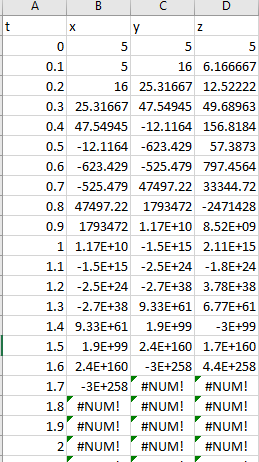
From the above result, it is observed that the solution of Lorentz equations by the Euler’s method with step size 0.1 the values are continuously decreasing. Hence, Euler method with step size 0.1 gives unstable solution for the Lorentz equations.
(b)
To calculate: The solution of Lorentz equation
Answer to Problem 18P
Solution:
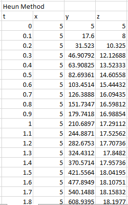
The solution of Lorentz equations by the Heun’s method with step size 0.1 gives unstable solution.
Explanation of Solution
Given Information:
Lorentz equations,
and Initial conditions are
Formula used:
The iteration formula for Heun’s method is,
Calculation:
Consider the equations,
The following VBA code is used to solve the Lorentz equation by Heun’s method:
Code:
Output:
To draw the graph of the above results, follow the steps in excel sheet as given below,
Step 1: Select the cell from A4 to A205 and cell B4 to B205. Then, go to the Insert and select the scatter with smooth lines from the chart.
Step 2: Select the cell from A4 to A205 and cell C4 to C205. Then, go to the Insert and select the scatter with smooth lines from the chart.
Step 2: Select the cell from A4 to A205 and cell D4 to D205. Then, go to the Insert and select the scatter with smooth lines from the chart.
Step 4: Select one of the graphs and paste it on another graph to merge the graphs.
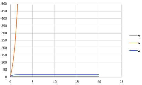
The graph obtained is,
And, to draw the phase plane plot follow the steps as below,
Step 4: Select the column B, column C and column D. Then, go to the Insert and select the scatter with smooth lines from the chart.
The graph obtained is,
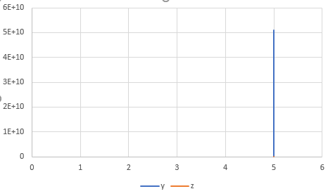
The phase plane plot is a straight line because solution of x is a constant value. The solution o0f Lorentz equation by Heun’s method with step size 0.1 is thus unstable.
(c)
To calculate: The solution of Lorentz equation
Answer to Problem 18P
Solution:
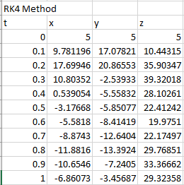
The first few solutions of Lorentz equation are,
| t | x | y | z |
| 0 | 5 | 5 | 5 |
| 0.1 | 9.781196 | 17.07821 | 10.44315 |
| 0.2 | 17.69946 | 20.86553 | 35.90347 |
| 0.3 | 10.80352 | -2.53933 | 39.32018 |
| 0.4 | 0.539054 | -5.55832 | 28.10261 |
| 0.5 | -3.17668 | -5.85077 | 22.41242 |
| 0.6 | -5.5818 | -8.41419 | 19.9751 |
| 0.7 | -8.8743 | -12.6404 | 22.17497 |
| 0.8 | -11.8816 | -13.3924 | 29.76851 |
| 0.9 | -10.6546 | -7.2405 | 33.36662 |
| 1 | -6.86073 | -3.45687 | 29.32358 |
Explanation of Solution
Given Information:
Lorentz equations,
and Initial conditions are
Formula used:
The fourth-order RK method for
Where,
Calculation:
The following VBA code is used to find the solution of Lorentz equation by the fourth order RK method:
Code:
Output:
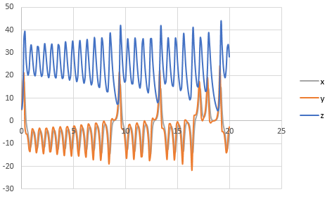
To draw the graph of the above results, follow the steps in excel sheet as given below,
Step 1: Select the cell from A4 to A205 and cell B4 to B205. Then, go to the Insert and select the scatter with smooth lines from the chart.
Step 2: Select the cell from A4 to A205 and cell C4 to C205. Then, go to the Insert and select the scatter with smooth lines from the chart.
Step 3: Select the cell from A4 to A205 and cell D4 to D205. Then, go to the Insert and select the scatter with smooth lines from the chart.
Step 4: Select one of the graphs and paste it on another graph to merge the graphs.
The graph obtained is,
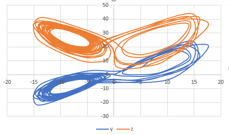
And, to draw the phase plane plot follow the steps as below,
Step 4: Select the column B, column C and column D. Then, go to the Insert and select the scatter with smooth lines from the chart.
The graph obtained is,
(d)
The solution of Lorentz equation
Answer to Problem 18P
Solution:
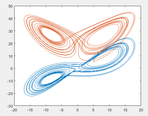
The solution graph of Lorentz equation is,
Explanation of Solution
Given Information:
Lorentz equations,
and Initial conditions are
Consider the Lorentz equations,
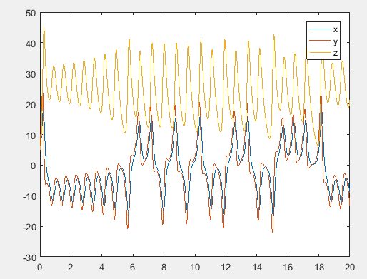
Use MATLAB ode45 function to solve the above differential functions as below,
Code:
Output:
The graph obtained as,
Write the command as below to plot the phase-plane,

The phase plane graph obtained as,
Want to see more full solutions like this?
Chapter 28 Solutions
EBK NUMERICAL METHODS FOR ENGINEERS
Additional Engineering Textbook Solutions
Advanced Engineering Mathematics
Basic Technical Mathematics
Fundamentals of Differential Equations (9th Edition)
Excursions in Modern Mathematics (9th Edition)
Precalculus: Mathematics for Calculus (Standalone Book)


- Question 4. Consider the instance F4 || Cmax Wwith no buffer (means jobs are not unload from previous machine until next machine is not available) in front of all machines except M1. Apply NEH Algorithm to minimize the Cmax Jobs 1 2 3 6 М1 17 13 29 23 37 31 М2 25 27 33 31 37 41 M 3 52 14 43 34 25 47 М4 28 31 48 43 18 17arrow_forwardA projectile is launched with a velocity of 100 m/s at an angle of 30° above the horizontal. Create a Simulink model to solve the projectile's equations of motion, where x and y are the horizontal and vertical displacements of the projectile. X=0 x(0) = 100 cos 30º x(0)=0 ÿ=-g y(0)=0 y(0)=100 sin 30º Use the model to plot the projectile's trajectory y versus x for 0≤t≤10 s.arrow_forwardResponse using Laplace transformation.arrow_forward
- The 2nd order ODE given below models the vertical fall of on Object under the influence of gravity and air friction md²y acceleration -mg + (1/2 Co A Pair) (dy) ² Forcing due logranty Forcing due to air frictionarrow_forwardA mechanical system is represented by two masses and three springs, where m, = 12 kg, m, = 22kg, and spring constants k, = k, = k, = 15 N/m, as shown in the following figure. k3 m2 Determine the largest eigenvalue of this mechanical system using the characteristic equation. a. b. Determine the smallest eigenvalue and the corresponding eigenvector using Inverse Power method. Given the initial eigenvector v(0)= (1 1 1). Iterate until | Ar41 - 1x 50.0005.arrow_forwardA// Use Implicit Method to solve the temperature distribution of a long thin rod with a length of 9 cm and following values: k = 0.49 cal/(s cm °C), Ax = 3 cm, and At = 0.2 s. At t=0 s, the temperature of the rod is 10°C and the boundary conditions are fixed dT (9,t) 1 °C/cm. Note that the rod for alltimes at 7(0,t) = 80°C and derivative condition dx is aluminum with C = 0.2174 cal/g °C) and p = 2.7 g/cm³. Find the temperature values on the inner grid points and the right boundary for t = 0.4 s.arrow_forward
- Write a brief (a few sentences) discussion about the significance of each of the following in regards to an iterative CFD solution: (a) initial conditions, (b) residual, (c) iteration, and (d) postprocessing.arrow_forwardHello, could I get some help with a Differential Equations problem that involves Eigenvalues and Eigenvectors? The set up is: There are two toy rail cars, Car 1, and Car 2. Car 1 has a mass of 2 kg, and is traveling 3 m/s towards Car 2, which has a mass of 1 kg, and is traveling towards Car 1 at 2 m/s. There is a bumper on the second rail car that engages at the moment the cars hit (connecting Car 1 and Car 2), and does not let go. The bumper acts like a spring with spring constant K = 2 N/m. Car 2 is 7 m from the wall at the time of collision (Car 2 is between Car 1 and the wall). I have attached the work I have done so far, but I'm not understanding how to find x1(t) and x2(t), how we know Car 2 hits the wall (or moves away from it), and at what speed Car 1 travels to stay in place after link-up (given: 1 m/s, but not sure why that is). Thank you in advance.arrow_forwardConsider the thermocouple properties you found in the question "Temperature of a thermocouple (1/3)" If the thermocouple is initially outside of the bath at room temperature (20 °C), what is the maximum temperature it will register if it's instantaneously inserted into the batch (55 °C) for 18 seconds and then removed? Use an inverse Laplace transform to find the solution. a. 32.68 °C b. 44.97 °C c. 64.97 °C d. 12.68 °Carrow_forward
- As4. This is my third time asking this question. Please DO NOT copy and paste someone else's work or some random notes. I need an answer to this question. There is a mass attached to a spring which is fixed against a wall. The spring is compressed and then released. Friction and is neglected. The velocity and displacement of the mass need to be modeled with an equation or set of equations so that various masses and spring constants can be input into Matlab and their motion can be observed. Motion after being released is only important, the spring being compressed is not important. This could be solved with dynamics, Matlab, there are multiple approaches.arrow_forwardThe governing equation of motion for a base motion system is given by (assume the units are Newton) mä(t)+ci(t)+kx(t) =cY@, cos(@,t) +kY sin(@t) %3D Given that m = 180 kg, c = 30 kg/s, Y = 0.02 m, and о, — 3.5 rad/s %3| 1. Use Excel or Matlab to find the largest value of the stiffness, k that makes the transmissibility ratio less than 0.85 2. Using the value of the stiffness obtained in part (1), determine the transmitted force to the base motion system using Matlab or Excel. 3. Display and discuss your results.arrow_forwardThe Gilles & Retzbach model of a distillation column, the system model includes the dynamics of a boiler, is driven by the inputs of steam flow and the flow rate of the vapour side stream, and the measurements are the temperature changes at two different locations along the column. The state space model is given by: x = 0 00 -30.3 0.00012 -6.02 0 0 0 -3.77 00 0 -2.80 0 0 Is the system?: a. unstable b. C. not unstable x+ 6.15 0 0 0 0 3.04 0 0.052 not asymptotically stable d. asymptotically stable -1 u y = 0 0 0 0 -7.3 0 0 -25.0 Xarrow_forward
 Elements Of ElectromagneticsMechanical EngineeringISBN:9780190698614Author:Sadiku, Matthew N. O.Publisher:Oxford University Press
 Mechanics of Materials (10th Edition)Mechanical EngineeringISBN:9780134319650Author:Russell C. HibbelerPublisher:PEARSON
 Thermodynamics: An Engineering ApproachMechanical EngineeringISBN:9781259822674Author:Yunus A. Cengel Dr., Michael A. BolesPublisher:McGraw-Hill Education
 Control Systems EngineeringMechanical EngineeringISBN:9781118170519Author:Norman S. NisePublisher:WILEY
 Mechanics of Materials (MindTap Course List)Mechanical EngineeringISBN:9781337093347Author:Barry J. Goodno, James M. GerePublisher:Cengage Learning
 Engineering Mechanics: StaticsMechanical EngineeringISBN:9781118807330Author:James L. Meriam, L. G. Kraige, J. N. BoltonPublisher:WILEY