
Concept explainers
Videos
The basic differential equation of the elastic curve for a uniformly loaded beam (Fig. P28.27) is given as
Where
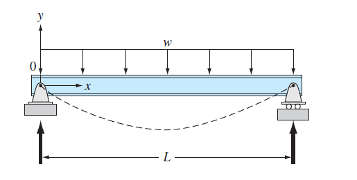
FIGURE P28.27
(a)
To calculate: The deflection of the beam by the finite-difference method with
Answer to Problem 27P
Solution:
The deflection of the beam by the finite-difference method is,
| x | y | y-Analytical |
| 0 | 0 | 0 |
| 24 | ||
| 48 | ||
| 72 | ||
| 96 | ||
| 120 | 0 | 0 |
Explanation of Solution
Given Information:
The differential equation for the elastic curve for a uniformly loaded beam is given as,
Formula to find analytical value,
Where,
The modulus of elasticity,
The moment of inertia,
The values,
Formula used:
The conversion formula,
The value of second order derivative by finite difference method is given as,
Calculation:
Consider the equation,
Rewrite the above equation as,
Substitute the values,
Now, the second order derivative by finite difference method gives,
Therefore,
Put
The boundary condition is,
Put
Substitute
Put
Substitute
Put
Substitute
The matrix form of the above equations is given as below,
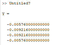
Use MATLAB to find the solution of the above system as below,
Code:
%Write the matrix
A=[-2 1 0 0; 1 -2 1 0; 0 1 -2 1; 0 0 1 -2];
%write the values of rhs
b=[0.002304 0.003456 0.003456 0.002304]';
%find the result
Y=A\b
Output:
Now, for the analytical value, consider the equation
Substitute the values,
Use excel to find the values of y at different values of x as below,
Step 1: Name the column A as x and go to column A2 and put 0 then go to column A3 and write the formula as,
=A2+24
Then, Press enter and drag the column up to
Step 2: Now name the column B as y and go to column B2 andwrite the formula as,
=2.89236*10^(-10)*A2*(120*A2^2-0.5*A2^3-864000)
Step 3: Press enter and drag the column up to
The result obtained as,
| x | y-Analytical |
| 0 | 0 |
| 24 | |
| 48 | |
| 72 | |
| 96 | |
| 120 | 0 |
(b)
To calculate: The deflection of the beam by the shooting method with
Answer to Problem 27P
Solution:
A few values of deflection of the beam by the shooting method is,
| x | y | z |
| 0 | 0 | -1.6E-06 |
| 0.25 | -4.1E-07 | -1.6E-06 |
| 0.5 | -8.2E-07 | -1.6E-06 |
| 0.75 | -1.2E-06 | -1.6E-06 |
| 1 | -1.6E-06 | -1.6E-06 |
| 1.25 | -2E-06 | -1.5E-06 |
| 1.5 | -2.4E-06 | -1.4E-06 |
| 1.75 | -2.8E-06 | -1.4E-06 |
| 2 | -3.2E-06 | -1.3E-06 |
| 2.25 | -3.5E-06 | -1.2E-06 |
| 2.5 | -3.8E-06 | -1.1E-06 |
| 2.75 | -4.1E-06 | -1E-06 |
| 3 | -4.4E-06 | -9E-07 |
Explanation of Solution
Given Information:
The differential equation for the elastic curve for a uniformly loaded beam is given as,
Formula to find analytical value,
Where,
The modulus of elasticity,
The moment of inertia,
The values,
Formula used:
The conversion formula,
Calculation:
Consider the equation,
Rewrite the equation as,
Assume
Substitute the values,
Use VBA program as below to solve the above differential equation as below,
Code:
OptionExplicit
'Create a function find
Subfind()
'declare the variables as integer
Dim n AsInteger, j AsInteger
'declare the variables as double
DimdydxAsDouble, x AsDouble, dy2dx AsDouble, yanalAsDouble, E AsDouble, I AsDouble, w AsDouble, L AsDouble
DimolddydxAsDouble, oldy AsDouble, y AsDouble, h AsDouble
'Set the values of the variables
E =30000
I =800
w =1
L =10
y =0
x =0
h =0.25
dydx=0
'store dydx and analytical solution
dydx= caldydx(w, E, I, L, x)
yanal= caly(w, E, I, L, x)
'use for loop to determine different value of y and y analytical
For j =1 To41
'store the value of y at oldy and dydx in olddydx
oldy = y
olddydx= dydx
'Store d2ydx, dydx and analytical solution
dy2dx = caldy2dx(w, E, I, L, x)
dydx= caldydx(w, E, I, L, x)
yanal= caly(w, E, I, L, x)
'move to the cell b3
Range("b1"). Select
ActiveCell.Value="shooting method"
'Assign name to the columns
ActiveCell.Offset(1,0). Select
ActiveCell.Value="x"
ActiveCell.Offset(0,1). Select
ActiveCell.Value="y"
ActiveCell.Offset(0,1). Select
ActiveCell.Value="z"
ActiveCell.Offset(0,1). Select
ActiveCell.Value="dy2dx"
ActiveCell.Offset(0,1). Select
ActiveCell.Value="y-anal"
'dislay values in cell
Range("b2"). Select
ActiveCell.Offset(j,0). Select
ActiveCell.Value= x
ActiveCell.Offset(0,1). Select
ActiveCell.Value= oldy
ActiveCell.Offset(0,1). Select
ActiveCell.Value= dydx
ActiveCell.Offset(0,1). Select
ActiveCell.Value= dy2dx
ActiveCell.Offset(0,1). Select
ActiveCell.Value= yanal
'Write the next value of x
x = x + h
'Write the next value of y by euler method
y = oldy + olddydx* h
Next
EndSub
'Define d2ydx function
Function caldy2dx(w, E, I, L, x)
'Declare the variables
Dim t AsDouble
'Write the formula
t =((w * L * x)/(2* E * I))-((w * x * x)/(2* E * I))
'Store the value
caldy2dx = t
EndFunction
'Define dydx
Functioncaldydx(w, E, I, L, x)
'Declare the variables
Dim t AsDouble, c AsDouble
'Set the values
c =-0.000001648
'Write the formula
t =((w * L * x * x)/(4* E * I))-((w * x * x * x)/(6* E * I))+ c
'Store the value
caldydx= t
EndFunction
'Define the function caly for analytical value
Functioncaly(w, E, I, L, x)
'Declare the variables
Dim t AsDouble
'Write the formula
t =((w * L * x * x * x)/(12* E * I))-((w * x * x * x * x)/(24* E * I))-((w * L * L * L * x)/(24* E * I))
'Store the value
caly= t
EndFunction
Output:
| shooting method | ||||
| x | y | z | dy2dx | y-anal |
| 0 | 0 | -1.6E-06 | 0 | 0 |
| 0.25 | -4.1E-07 | -1.6E-06 | 5.08E-08 | -4.3E-07 |
| 0.5 | -8.2E-07 | -1.6E-06 | 9.9E-08 | -8.6E-07 |
| 0.75 | -1.2E-06 | -1.6E-06 | 1.45E-07 | -1.3E-06 |
| 1 | -1.6E-06 | -1.6E-06 | 1.88E-07 | -1.7E-06 |
| 1.25 | -2E-06 | -1.5E-06 | 2.28E-07 | -2.1E-06 |
| 1.5 | -2.4E-06 | -1.4E-06 | 2.66E-07 | -2.5E-06 |
| 1.75 | -2.8E-06 | -1.4E-06 | 3.01E-07 | -2.9E-06 |
| 2 | -3.2E-06 | -1.3E-06 | 3.33E-07 | -3.2E-06 |
| 2.25 | -3.5E-06 | -1.2E-06 | 3.63E-07 | -3.6E-06 |
| 2.5 | -3.8E-06 | -1.1E-06 | 3.91E-07 | -3.9E-06 |
| 2.75 | -4.1E-06 | -1E-06 | 4.15E-07 | -4.2E-06 |
| 3 | -4.4E-06 | -9E-07 | 4.38E-07 | -4.4E-06 |
| 3.25 | -4.7E-06 | -7.9E-07 | 4.57E-07 | -4.6E-06 |
| 3.5 | -4.9E-06 | -6.7E-07 | 4.74E-07 | -4.8E-06 |
| 3.75 | -5.1E-06 | -5.5E-07 | 4.88E-07 | -5E-06 |
| 4 | -5.2E-06 | -4.3E-07 | 5E-07 | -5.2E-06 |
| 4.25 | -5.4E-06 | -3E-07 | 5.09E-07 | -5.3E-06 |
| 4.5 | -5.5E-06 | -1.7E-07 | 5.16E-07 | -5.4E-06 |
| 4.75 | -5.6E-06 | -4.2E-08 | 5.2E-07 | -5.4E-06 |
| 5 | -5.6E-06 | 8.81E-08 | 5.21E-07 | -5.4E-06 |
| 5.25 | -5.6E-06 | 2.18E-07 | 5.2E-07 | -5.4E-06 |
| 5.5 | -5.6E-06 | 3.48E-07 | 5.16E-07 | -5.4E-06 |
| 5.75 | -5.5E-06 | 4.76E-07 | 5.09E-07 | -5.3E-06 |
| 6 | -5.4E-06 | 6.02E-07 | 5E-07 | -5.2E-06 |
| 6.25 | -5.3E-06 | 7.26E-07 | 4.88E-07 | -5E-06 |
| 6.5 | -5.2E-06 | 8.46E-07 | 4.74E-07 | -4.8E-06 |
| 6.75 | -5E-06 | 9.62E-07 | 4.57E-07 | -4.6E-06 |
| 7 | -4.8E-06 | 1.07E-06 | 4.38E-07 | -4.4E-06 |
| 7.25 | -4.5E-06 | 1.18E-06 | 4.15E-07 | -4.2E-06 |
| 7.5 | -4.3E-06 | 1.28E-06 | 3.91E-07 | -3.9E-06 |
| 7.75 | -4E-06 | 1.38E-06 | 3.63E-07 | -3.6E-06 |
| 8 | -3.7E-06 | 1.46E-06 | 3.33E-07 | -3.2E-06 |
| 8.25 | -3.3E-06 | 1.54E-06 | 3.01E-07 | -2.9E-06 |
| 8.5 | -3E-06 | 1.61E-06 | 2.66E-07 | -2.5E-06 |
| 8.75 | -2.6E-06 | 1.68E-06 | 2.28E-07 | -2.1E-06 |
| 9 | -2.2E-06 | 1.73E-06 | 1.88E-07 | -1.7E-06 |
| 9.25 | -1.7E-06 | 1.77E-06 | 1.45E-07 | -1.3E-06 |
| 9.5 | -1.3E-06 | 1.8E-06 | 9.9E-08 | -8.6E-07 |
| 9.75 | -8.7E-07 | 1.82E-06 | 5.08E-08 | -4.3E-07 |
| 10 | -4.2E-07 | 1.82E-06 | 0 | 0 |
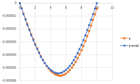
Now, to draw the graph of y and y-analytical follow the step as below,
Step 1: Select the cell from B2 to B43 and cell C2 to C43. Then, go to the Insert and select the scatter with smooth lines from the chart.
Step 2: Select the cell from B2 to B43 and cell F2 to F43. Then, go to the Insert and select the scatter with smooth lines from the chart.
Step 3: Select one of the graphs and paste it on another graph to merge the graphs.
The graph obtained is,
Want to see more full solutions like this?
Chapter 28 Solutions
EBK NUMERICAL METHODS FOR ENGINEERS
Additional Engineering Textbook Solutions
Fundamentals of Differential Equations (9th Edition)
Advanced Engineering Mathematics
Basic Technical Mathematics


- Creep exercises The following data in the table below was obtained a from rupture test. Stress (MPa) Temperature (°C) Rupture time (hr) T 550 580 0.75 550 555 5.5 550 540 19.2 550 525 62.0 70 760 2.05 70 730 8.2 70 700 36.5 70 675 134 Assume: C = 46 Establish whether the Larson-Miller parameter is valid for both stresses (550 and 70 MPa). Was there a change in creep mechanism when changing the stress from 550 to 70 MPa during rupture test? Motivate your answer with the aid of calculation.arrow_forwardA Cantilever beam deflects downwards when a mass is attached to its free end. The deflection (8) is the function of beam stiffness(K), applied mass(M) and gravitational force(g=9.81 m/s2): K8=Mg Determine the stiffness of beam? The various mass are placed on the end of the beam and corresponding deflections are noted as follow: 150.05 200.05 Mass Deflection 0 0 50.15 99.90 0.6 1.8 3.0 3.6 using the "Correlation Coefficient" equation, check whether the 'line-fitting' has; (i) strong positive linear relationship (ii) strong negative linear relationship (iii) no linear relationship 250.20 299.95 350.05 401.00 4.8 6.0 6.2 7.5arrow_forward22°F Clear 1MMBU BU ► ► ► 20°HD®°°*EqqaHÛDin × ODE DDE DE DE File C:/Users/ignor/Downloads/Assignment%203%20(2).pdf T❘ Read aloud Ask Copilot Draw a) Use Newton's second law b) Use the Torque equation /// Collar A is free to slide with negligible friction on the circular guide mounted in a vertical frame. Find the EOM of collar A if the frame is given a velocity v and a constant horizontal acceleration a to the right. Search 1 A www of 6 TTTT | CD a laaa 8 o + ENG 60 T N 7:35 PM 1/17/2024 xarrow_forward
- 1. In the test-firing of a missile, there are some events that are known to cause the missile to fail to reach its target. These events are listed below, together with their approximate probabilities of occurrence during a flight: Event Probability (A1) Cloud reflection (A2) Precipitation (A3) Target evasion (A4) Electronic countermeasure 0.0001 0.005 0.002 0.04 The probabilities of failure if these events occur are: F F G) = 0.3; P| G) = 0.01; P | 이-)= 0.005; P = 0.0002 Use Bayes' theorem (Eq. 2.10) to calculate the probability of each of these events being the cause in the event of a missile failing to reach its target. Bayes' theorem: P(B|A) * P(A) P(A|B) = P(B)arrow_forward1. The cross section foresights at one station along a proposed highway are shown below. The HI for these foresights is 970.61 ft. Plot the cross section elevation to scale. 5.2 4.8 6.6 5.9 7.0 8.1 24 + 00 50 22 0 12 30 50 2. The roadway subgrade elevation is 973.30 ft., the planned roadbed is 30-feet wide, with side slopes of 2%:1. Plot the roadbed design elevations on the plot from problem 1, and find the slope intercepts and the cross section area. 3. The cross section foresights for the next station are show below. They were observed from the same instrument setup as in problem 1. The subgrade elevation is 972.30 ft. Use the same roadbed width and side slopes from problem 2. Plot the cross section and the roadbed elevations to scale, find the slope intercepts, and find the cross section area. 4.8 25 + 00 3.2 5.3 50 0 50 4. What is the volume of soil to be removed or added between stations 24 and 25? Hint: To calculate volume of soil between stations 24+00 and 25+00 Use the…arrow_forward5. A beam has a square cross-section, a x a, where a is the linear dimension, and is subject to a pure bending moment, M. M is known with an uncertainty of +8% and a is known with an uncertainty of +9%. The strength of the material is known to an uncertainty of ±5%. Find the minimum design factor such that the beam is guaranteed not to fail. Note that this is a beam in bending, not a link in tension, so the stress equation is different from what was presented in class. Remember ME 3403.arrow_forward
- A long steel rod is placed horizontally between two supports, one at each end. The rod bends a little in the center. Which property of this rod can be used to estimate how much the rod should bend at the center? 1. Its Shear Modulus 2. Its Young's Modulus 3. All of these Moduli can be used to compute how much it bends. 4. Its Bulk Modulus.arrow_forwardb) In an engine design, a pair of bearing is designed to carry low load. If the lifetime of the pair of identical gear obey Weibull distribution with random with parameter a=0.0002 and B=0.5. %23 (b) Find the probability that both bearings functions properly at least 6000 hours. ::. :.arrow_forwardWhat mathematical relationship exists between the wave speed and the density of the medium, using the POWER trendline equation from the graph? Make your response specific (i.e., describe the full mathematical proportionality between the two variables) Feel free to use the table. Table: Frequency (Hz) Density (kg/m) Tension (N) Speed (cm/s) Wavelength (cm) 0.85 0.1 4.0 632.5 744.12 0.85 0.7 4.0 239.0 281.18 0.85 1.3 4.0 175.4 206.35 0.85 1.9 4.0 145.1 170.70arrow_forward
- Find the mobility, the Grashof condition, and the Barker classification of the following oil field pump. 76 51.26 47.5 14 80 12arrow_forwardH WebAssign - ENGR 2331 Su2 x A 23 Changes in Lengths unde x yL.Het/web/Student/Assignment-Responses/last?dep326956848#Q3 : Apps M Gmail YouTube O Maps DETAILS UUMECHMATI Z.3.UT7. MT NOTES ASK TOUK TEACHEK A flat bar of rectangular cross section, length L, and constant thickness t is subjected to tension by forces P (see figure). b2 P b1 The width of the bar varies linearly from b, at the smaller end to b, at the larger end. Assume that the angle of taper is small. (a) Derive the following formula for the elongation of the bar. (Submit a file with a maximum size of 1 MB.) PL Et(b, - Choose File No file chosen This answer has not been graded yet. (b) Calculate the elongation (in inches), assuming L = 3 ft, t = 1.0 in., P = 23 kips, b, = 4.0 in., b, = 5.4 in., and E = 30 x 106 psi. (Use the deformation sign convention.) in. 73°F Partly sunny Watch it Need Help2 Read It O Type here to search hparrow_forwardDerive the rule-of-mixtures expression for the composite extensional modulus E₁ assuming the existence of an interphase region. The starting point for the derivation would be the model shown below. For simplicity, assume the interphase, like the matrix, is isotropic with modulus E¹. With an interphase region there is a volume fraction associated with the interphase (i.e.,V;). For this situation: vf + vm + Vi = 1 wi |||||||arrow_forward
 Elements Of ElectromagneticsMechanical EngineeringISBN:9780190698614Author:Sadiku, Matthew N. O.Publisher:Oxford University Press
 Mechanics of Materials (10th Edition)Mechanical EngineeringISBN:9780134319650Author:Russell C. HibbelerPublisher:PEARSON
 Thermodynamics: An Engineering ApproachMechanical EngineeringISBN:9781259822674Author:Yunus A. Cengel Dr., Michael A. BolesPublisher:McGraw-Hill Education
 Control Systems EngineeringMechanical EngineeringISBN:9781118170519Author:Norman S. NisePublisher:WILEY
 Mechanics of Materials (MindTap Course List)Mechanical EngineeringISBN:9781337093347Author:Barry J. Goodno, James M. GerePublisher:Cengage Learning
 Engineering Mechanics: StaticsMechanical EngineeringISBN:9781118807330Author:James L. Meriam, L. G. Kraige, J. N. BoltonPublisher:WILEY