
Introduction To Statistics And Data Analysis
6th Edition
ISBN: 9781337793612
Author: PECK, Roxy.
Publisher: Cengage Learning,
expand_more
expand_more
format_list_bulleted
Videos
Textbook Question
Chapter 7.7, Problem 108E
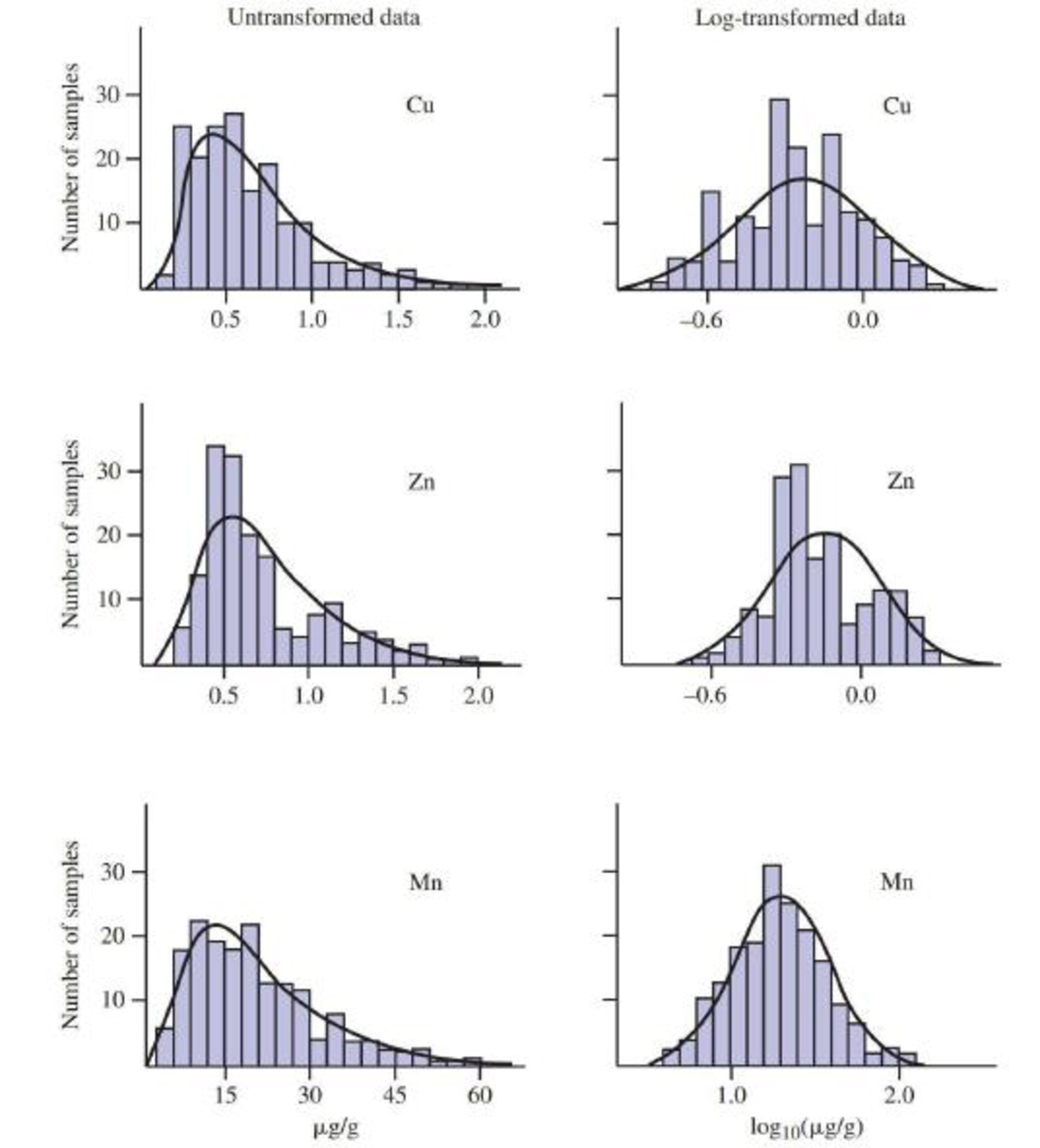
The figure on the next page appeared in the paper “EDTA-Extractable Copper, Zinc, and Manganese in Soils of the Canterbury Plains” (New Zealand Journal of Agricultural Research [1984]: 207–217). A large number of topsoil samples were analyzed for manganese (Mn), zinc (Zn), and copper (Cu), and the resulting data were summarized using histograms.
The investigators transformed each data set using logarithms in an effort to obtain more nearly symmetric distributions of values. Do you think the transformations were successful? Explain.
Expert Solution & Answer
Want to see the full answer?
Check out a sample textbook solution
Students have asked these similar questions
Because of high tuition costs at state and private universities, enrollments atcommunity colleges have increased dramatically in recent years. The following data show theenrollment (in thousands) for Jefferson Community College from 2001–2009:Year Period (t) Enrollment (1000s)2001 1 6.52002 2 8.12003 3 8.42004 4 10.22005 5 12.52006 6 13.32007 7 13.72008 8 17.22009 9 18.1Compute F10: the Forecast for 2010. Compute Pearson’s Correlation Coefficient Use the Method of Least Squares to obtain the Best-Fit-Line for this data. Use the line to compute the forecast.
2.62 For the period 2001–2008, the Bristol-Myers Squibb Company, Inc. reported the following amounts (in billions of dollars) for (1) net sales and (2) advertising and product promotion. The data are also in the file XR02062.
Source: Bristol-Myers Squibb Company, Annual Reports, 2005, 2008.
Year Net Sales Advertising/Promotion
2001 $16.612 $1.201
2002 16.208 1.143
2003 18.653 1.416
2004 19.380 1.411
2005 19.207 1.476
2006 16.208 1.304
2007 18.193 1.415
2008 20.597 1.550
For these data, construct a line graph that shows both net sales and expenditures for advertising/product promotion over time. Some would suggest that increases in advertising should be accompanied by increases in sales. Does your line graph support this?
1. An article in Air and Waste (“Update on Ozone Trends in California’s South Coast Air Basin,” Vol. 43, 1993) studied the ozone levels on the South Coast air basin of California for the years 1976–1991. The author believes that the number of days that the ozone level exceeds 0.20 parts per million depends on the seasonal meteorological index (the seasonal average 850 millibar temperature). The data follow:(a) Construct a scatter diagram of the data.(b) Fit a simple linear regression model to the data. (c) Compute for the correlation coefficient. What trend does it follow?
Chapter 7 Solutions
Introduction To Statistics And Data Analysis
Ch. 7.1 - State whether each of the following random...Ch. 7.1 - Classify each of the following random variables as...Ch. 7.1 - Starting at a particular time, each car entering...Ch. 7.1 - A point is randomly selected from the interior of...Ch. 7.1 - A point is randomly selected on the surface of a...Ch. 7.1 - Prob. 6ECh. 7.1 - A box contains four slips of paper marked 1, 2, 3,...Ch. 7.2 - Define the random variable x to be the number of...Ch. 7.2 - Using the probability distribution given in the...Ch. 7.2 - Let y denote the number of broken eggs in a...
Ch. 7.2 - Use the probability distribution given in the...Ch. 7.2 - Suppose that fund-raisers at a university call...Ch. 7.2 - Airlines sometimes overbook flights. Suppose that...Ch. 7.2 - Suppose that a computer manufacturer receives...Ch. 7.2 - Simulate the chance experiment described in the...Ch. 7.2 - Of all airline flight requests received by a...Ch. 7.2 - Suppose that 20% of all homeowners in an...Ch. 7.2 - A box contains five slips of paper, marked 1, 1,...Ch. 7.2 - Components coming off an assembly line are either...Ch. 7.2 - When applying for a building permit, a contractor...Ch. 7.2 - A library subscribes to two different weekly news...Ch. 7.3 - Let x denote the lifetime (in thousands of hours)...Ch. 7.3 - Using the density curve for fan lifetime given in...Ch. 7.3 - A particular professor never dismisses class...Ch. 7.3 - Refer to the probability distribution given in the...Ch. 7.3 - The article Probabilistic Risk Assessment of...Ch. 7.3 - Use the density curve of x = distance of actual...Ch. 7.3 - Let x denote the amount of gravel sold (in tons)...Ch. 7.3 - Use the density curve for x = amount of gravel...Ch. 7.3 - Let x be the amount of time (in minutes) that a...Ch. 7.3 - Ref erring to the previous exercise, let x and y...Ch. 7.3 - The density curve for the random variable w (the...Ch. 7.4 - Consider selecting a household in rural Thailand...Ch. 7.4 - Suppose the probability distribution of x, the...Ch. 7.4 - Consider the following probability distribution...Ch. 7.4 - Referring to the previous exercise, use the result...Ch. 7.4 - Exercise 7.8 gave the following probability...Ch. 7.4 - Prob. 38ECh. 7.4 - Prob. 39ECh. 7.4 - Refer to the information given in Exercise 7.39....Ch. 7.4 - Refer to the information given in Exercise 7.39....Ch. 7.4 - Suppose that for a particular computer...Ch. 7.4 - A local television station sells 15-second,...Ch. 7.4 - An author has written a book and submitted it to a...Ch. 7.4 - A grocery store has an express line for customers...Ch. 7.4 - An appliance dealer sells three different models...Ch. 7.4 - To assemble a piece of furniture, a wood peg must...Ch. 7.4 - A multiple-choice exam consists of 50 questions....Ch. 7.4 - Consider a game in which a red die and a blue die...Ch. 7.4 - Consider the random variables xR and xB defined in...Ch. 7.5 - CBS News reported that 4% of adult Americans have...Ch. 7.5 - Flight View surveyed 2600 North American airline...Ch. 7.5 - Refer to the previous exercise, and suppose that...Ch. 7.5 - Twenty-five percent of the customers of a grocery...Ch. 7.5 - Example 7.18 described a study in which a person...Ch. 7.5 - Information Security Buzz provides news for the...Ch. 7.5 - A breeder of show dogs is interested in the number...Ch. 7.5 - Womens Health Magazine surveyed 1187 readers to...Ch. 7.5 - Prob. 60ECh. 7.5 - Suppose that the probability is 0.1 that any given...Ch. 7.5 - Suppose that 30% of all automobiles undergoing an...Ch. 7.5 - Suppose that you will take a multiple-choice exam...Ch. 7.5 - Suppose that 20% of the 10,000 signatures on a...Ch. 7.5 - A city requires that smoke detectors be installed...Ch. 7.5 - Suppose that 90% of all registered California...Ch. 7.5 - Suppose a playlist on a music player consists of...Ch. 7.5 - Sophie is a dog that loves to play catch....Ch. 7.5 - Suppose that 5% of cereal boxes contain a prize...Ch. 7.6 - Determine the following standard normal (z) curve...Ch. 7.6 - Determine the following standard normal (z) curve...Ch. 7.6 - Determine each of the following areas under the...Ch. 7.6 - Determine each of the following areas under the...Ch. 7.6 - Let z denote a random variable that has a standard...Ch. 7.6 - Let z denote a random variable that has a standard...Ch. 7.6 - Let z denote a random variable having a normal...Ch. 7.6 - Let z denote a random variable having a normal...Ch. 7.6 - Let z denote a variable that has a standard normal...Ch. 7.6 - Determine the value z that a. Separates the...Ch. 7.6 - Determine the value of z such that a. z and z...Ch. 7.6 - Because P(z 0.44) = 0.67, 67% of all z values are...Ch. 7.6 - Consider the population of all 1-gallon cans of...Ch. 7.6 - Consider babies born in the normal range of 3743...Ch. 7.6 - Use the information on birth weights for babies...Ch. 7.6 - Emissions of nitrogen oxides, which are major...Ch. 7.6 - The paper referenced in Example 7.30 (Estimating...Ch. 7.6 - The size of the left upper chamber of the heart is...Ch. 7.6 - The paper referenced in the previous exercise also...Ch. 7.6 - The article New York Citys Graffiti-Removal...Ch. 7.6 - A machine that cuts corks for wine bottles...Ch. 7.6 - Refer to the previous exercise. Suppose that there...Ch. 7.6 - Purchases made at small corner stores were studied...Ch. 7.6 - The time that it takes a randomly selected job...Ch. 7.6 - Suppose that the distribution of typing speed in...Ch. 7.6 - Consider the typing speed distribution described...Ch. 7.6 - Consider the typing speed distribution described...Ch. 7.7 - The authors of the paper Development of...Ch. 7.7 - The paper Risk Behavior, Decision Making, and...Ch. 7.7 - Prob. 99ECh. 7.7 - Prob. 100ECh. 7.7 - Macular degeneration is the most common cause of...Ch. 7.7 - The following normal probability plot was...Ch. 7.7 - Consider the following 10 observations on the...Ch. 7.7 - Prob. 104ECh. 7.7 - Prob. 105ECh. 7.7 - Prob. 106ECh. 7.7 - Prob. 107ECh. 7.7 - The figure on the next page appeared in the paper...Ch. 7.8 - Let x denote the IQ of an individual selected at...Ch. 7.8 - Suppose that the distribution of x = the number of...Ch. 7.8 - The number of vehicles leaving a turnpike at a...Ch. 7.8 - Suppose that x has a binomial distribution with n...Ch. 7.8 - Prob. 113ECh. 7.8 - Prob. 114ECh. 7.8 - Prob. 115ECh. 7.8 - Suppose that 70% of the bicycles sold by a certain...Ch. 7.8 - Suppose that 25% of the fire alarms in a large...Ch. 7.8 - Suppose that 65% of all registered voters in a...Ch. 7.8 - Flashlight bulbs manufactured by a certain company...Ch. 7.8 - A company that manufactures mufflers for cars...Ch. 7 - Let x denote the duration of a randomly selected...Ch. 7 - A soft-drink machine dispenses only regular Coke...Ch. 7 - A business has six customer service telephone...Ch. 7 - Prob. 124CRCh. 7 - Refer 10 the probability distribution given in...Ch. 7 - A new batterys voltage may be acceptable (A) or...Ch. 7 - A pizza company advertises that it puts 0.5 pounds...Ch. 7 - Suppose that fuel efficiency for a particular...Ch. 7 - A coin is flipped 25 times. Let x be the number of...Ch. 7 - The probability distribution of x, the number of...Ch. 7 - The amount of time spent by a statistical...Ch. 7 - The lifetime of a certain brand of battery is...Ch. 7 - A machine producing vitamin E capsules operates so...Ch. 7 - The Wall Street Journal (February 15, 1972)...Ch. 7 - The longest run of Ss in the sequence SSFSSSSFFS...Ch. 7 - Four peoplea, b, c, and dare waiting to give...Ch. 7 - Kyle and Lygia are going to play a series of...Ch. 7 - Suppose that your statistics professor tells you...Ch. 7 - Suppose that the pH of soil samples taken from a...Ch. 7 - The lightbulbs used to provide exterior lighting...Ch. 7 - Suppose there are approximately 40,000 travel...Ch. 7 - Prob. 2CRECh. 7 - Prob. 3CRECh. 7 - Prob. 5CRECh. 7 - Prob. 6CRECh. 7 - Two shipping services offer overnight delivery of...Ch. 7 - Prob. 8CRECh. 7 - Prob. 9CRECh. 7 - The Cedar Rapids Gazette (November 20, 1999)...Ch. 7 - Prob. 11CRECh. 7 - The article Men, Women at Odds on Gun Control...Ch. 7 - Suppose that a new Internet company Mumble.com...Ch. 7 - Refer to the previous exercise. Suppose that...Ch. 7 - A chemical supply company currently has in stock...Ch. 7 - Prob. 16CRECh. 7 - An experiment was conducted to investigate whether...Ch. 7 - A machine that produces ball bearings has...Ch. 7 - Consider the variable x = time required for a...Ch. 7 - The accompanying data on x = student-teacher ratio...Ch. 7 - Prob. 21CRE
Knowledge Booster


Learn more about
Need a deep-dive on the concept behind this application? Look no further. Learn more about this topic, statistics and related others by exploring similar questions and additional content below.Similar questions
- Researchers collected data to examine the relationship between pollutants and preterm births in Southern California. During the study air pollution levels were measured by air quality monitoring stations. Specifically, levels of carbon monoxide were recorded in parts per million, nitrogen dioxide and ozone in parts per hundred million, and coarse particulate matter PM10 in µg/m3. Length of gestation data were collected on 143,196 births between the years 1989 and 1993, and air pollution exposure during gestation was calculated for each birth. The analysis suggested that increased ambient PM10 and, to a lesser degree, CO concentrations may be associated with the occurrence of preterm births. a. The paragraph above describes an O A. Observational Study B. Experiment b. The cases in this research are OA. Air pollution exposure during gestation B. Each birth between 1989 and 1993 C. Each type of pollution measured by air quality monitoring stations D. Each year between 1989 and 1993 c.…arrow_forwardA prospective cohort study is run to estimate the incidence of stroke in persons 55 years of age and older. All participants are free of stroke at study start. Each participant is followed for a maximum of 5 years. The data are summarized in Table 3–14. Number of Strokes Number of Stroke-Free Person-Years Men (n = 125) 9 478 Women (n = 200) 21 97 What is the annual incidence rate of stroke in men? What is the annual incidence rate of stroke in women? What is the annual incidence rate of stroke (men and women combined)?arrow_forwardAn article reported on a study in which each of 13 workers was provided with both a conventional shovel and a shovel whose blade was perforated with small holes. The authors of the cited article provided the following data on energy expenditure [kcal/kg(subject)/lb(clay)]. Worker: 2 4 5 6 Conventional: 0.0015 0.0015 0.0018 0.0022 0.001 0.0016 0.0028 Perforated: 0.0015 0.001 0.0019 0.0013 0.0011 0.0017 0.0024 Worker: 10 11 12 13 Conventional: 0.0021 0.0015 0.0014 0.0023 0.0017 0.002 Perforated: 0.0021 0.0013 0.0013 0.0017 0.0015 0.0013 n USE SALT Do these data provide convincing evidence that the mean energy expenditure using the conventional shovel exceeds that using the perforated shovel? Test the relevant hypotheses using a significance level of 0.05. (Use SALT to calculate the P-value. Use Hd = Hconventional - Hperforated Round your test statistic to one decimal place and your P-value to three decimal places.) t= df = p-value = State your conclusion. O we fail to reject H,. We have…arrow_forward
- An article in Air and Waste ("Update on Ozone Trends in California's South Coast Air Basin," Vol. 43, 1993) studied the ozone levels on the South Coast air basin of California for the years 1976-1991. The author believes that the number of days that the ozone exceeds 0.20 parts per million depends on the seasonal meteorological index (the seasonal average 850 millibar temperature). The data follow: Year Days Index 16.3 1976 91 1977 105 17.1 1978 106 18.2 1979 108 18.1 1980 88 17.2 1981 91 18.2 1982 58 16.0 1983 82 17.2 Round your answers to 2 decimal places. (a) Fit a simple linear regression model to the data. Test for significance of regression using a = 0.05. y = i Calculate fo: i Year Days Index 1984 82 17.7 1985 65 17.2 1986 61 16.9 1987 48 17.1 1988 61 18.2 1989 43 17.3 1990 33 17.5 1991 36 16.6 i + i Is the simple linear regression model significant? No. (b) Calculate a 95% confidence interval on the slope. ≤B₁ ≤i Xarrow_forwardA study was performed looking at the risk of fractures in three rural Iowa communities according to whether their drinking water was “higher calcium,” “higher fluorides,” or “control” as determined by water samples. Table 11.10 presents data comparing the rate of fractures (over 5 years) between the higher-calcium vs the control communities for women ages 20–35 and 55–80, respectively . Table 11.10 Relationship of calcium content of drinking water to the rate of fractures in rural Iowa Ages 20-35 Number of women with fractures Total number of women Ages 55-80 Number of woemn with fractures Total number of women Control 3 37 Control 11 121 High calcium 1 33 High calcium 21 148 13.1 What test can be used to compare the fracturerates in these two communities while controlling for age? 13.2 Implement the test in Problem 13.1, report a p-value, and make a conclusion on relationship between drinking water calcium concentration and rate of fracture based on the p-value. 13.3…arrow_forwardA study was performed looking at the risk of fractures in three rural Iowa communities according to whether their drinking water was “higher calcium,” “higher fluorides,” or “control” as determined by water samples. Table 11.10 presents data comparing the rate of fractures (over 5 years) between the higher-calcium vs the control communities for women ages 20–35 and 55–80, respectively . Table 11.10 Relationship of calcium content of drinking water to the rate of fractures in rural Iowa Ages 20-35 Number of women with fractures Total number of women Ages 55-80 Number of woemn with fractures Total number of women Control 3 37 Control 11 121 High calcium 1 33 High calcium 21 148 13.1 What test can be used to compare the fracturerates in these two communities while controlling for age? 13.2 Implement the test in Problem 13.1, report a p-value, and make a conclusion on relationship between drinking water calcium concentration and rate of fracture based on the p-value.arrow_forward
- The table below shows the estimated vaccination coverage of adolescents aged 13-17 years, as reported in national surveys in 2020 and 2021. Vaccine Percent vaccinated (95% CI) Tdap (tetanus, diphtheria, and acellular pertussis vaccine) 2020: 90.1 (89.2–90.9) 2021: 89.6 (88.6–90.5) MMR (measles, mumps, and rubella vaccine) 2020: 92.4 (91.6–93.2) 2021: 92.2 (91.2–93.2) HPV (human papillomavirus vaccine) 2020: 58.6 (57.3–60.0) 2021: 61.7 (60.2–63.2) Answer these: a. For which vaccine(s) was there a statistically significant change in coverage from 2020 to 2021? For each, note whether it was a statistically significant increase or decrease? b. For which vaccine(s) was there no significant change in coverage from 2020 to 2021?arrow_forwardIf three of the quarterly seasonal indices for a set of data are 0.7,0.7, and 0.7, then the fourth seasonal index is equal to 1.4 a) TRUE b) FALSE Submit Answer format: Text The forecast with out seasonality is modeled as: Sales = 6 *t + 236.00, where t= time in months, beginning in January 2015. Seasonality for the first three months are given in the table below. Determine a seasonalized forecast for Feb of 2016. Month Seasonal Factor January 1.9000 February 0.6262 March 0.1000 Submit Answer format: Number: Round to: 1 decimal places.arrow_forward2) El-Harbawi and Babba' reported the data presented in the below table involving the toxicity of surfactant to the early stage marine fish, Grouper fish. Concentration of Number of Number of fish surfactant (mg/L) mortality 0.032 10 0.15 10 0.5 1.15 10 1 10 3 2 10 3.17 10 10 10 10 a. Plot the percentage of fish affected versus the natural logarithm of the dose and then find the lethal concentration which kill 50% of the fish, b. Convert the mortality percent to probit variables c. Find the linear equation that fits the data.arrow_forward
- rofessor Cornish studied rainfall cycles and sunspot cycles. (Reference: Australian Journal of Physics, Vol. 7, pp. 334-346.) Part of the data include amount of rain (in mm) for 6-day intervals. The following data give rain amounts for consecutive 6-day intervals at Adelaide, South Australia. 7 28 7 1 69 3 1 4 22 7 16 4 54 160 60 73 27 3 3 1 7 144 107 4 91 44 1 8 4 22 4 59 116 52 4 155 42 24 11 43 3 24 19 74 26 63 110 39 34 71 52 39 8 0 15 2 14 9 1 2 4 9 6 10 (i) Find the median. (Use 1 decimal place.)(ii) Convert this sequence of numbers to a sequence of symbols A and B, where A indicates a value above the median and B a value below the median. Test the sequence for randomness about the median at the 5% level of significance. (b) Find the number of runs R, n1, and n2. Let n1 = number of values above the median and n2 = number of values below the median. R n1 n2 (c) In the case, n1 > 20, we cannot use Table 10 of Appendix II to find the critical…arrow_forwardCardiovascular Disease Suppose the incidence rate of myocardial infarction (MI) was 5 per 1000 among 45- to 54-year-old men in 2000. To look at changes in incidence over time, 5000 men in this age group were followed for 1 year starting in 2010. Fifteen new cases of MI were found. Suppose that 25% of patients with Mi in 2000 died within 24 hours. This propartion is called the 24-hour case-fatality rate. Of the 15 new MI cases in the preceding study. 5 died within 24 hours. Test whether the 24-hour case- fatality rate changed from 2000 to 2010.arrow_forwardAn article in the journal Air and Waste (Update on Ozone Trends in California's South Coast Air Basin, Vol. 43, 1993) investigated the ozone levels in the South Coast Air Basin of California for the years 1976-1991. The author believes that the number of days the ozone levels exceeded 0.20 ppm (the response) depends on the seasonal meteorological index, which is the seasonal average 850-millibar Temperature (the predictor). The following table gives the data. Year Index 1976 1977 1978 1979 1980 1981 1982 1983 1984 1985 1986 1987 1988 1989 1990 1991 Days 91 105 106 108 88 91 58 82 81 65 61 48 61 43 33 36 16.7 17.1 18.2 18.1 17.2 18.2 16.0 17.2 18.0 17.2 16.9 17.1 18.2 17.3 17.5 16.6 (a) Construct a scatter diagram of the data. (b) Estimate the prediction equation. (c) Test for significance of regression. (d) Calculate the 95% CI and PI on for a seasonal meteorological index value of 17. Interpret these quantities.arrow_forward
arrow_back_ios
SEE MORE QUESTIONS
arrow_forward_ios
Recommended textbooks for you
 MATLAB: An Introduction with ApplicationsStatisticsISBN:9781119256830Author:Amos GilatPublisher:John Wiley & Sons Inc
 Probability and Statistics for Engineering and th...StatisticsISBN:9781305251809Author:Jay L. DevorePublisher:Cengage Learning
 Statistics for The Behavioral Sciences (MindTap C...StatisticsISBN:9781305504912Author:Frederick J Gravetter, Larry B. WallnauPublisher:Cengage Learning
 Elementary Statistics: Picturing the World (7th E...StatisticsISBN:9780134683416Author:Ron Larson, Betsy FarberPublisher:PEARSON
 The Basic Practice of StatisticsStatisticsISBN:9781319042578Author:David S. Moore, William I. Notz, Michael A. FlignerPublisher:W. H. Freeman
 Introduction to the Practice of StatisticsStatisticsISBN:9781319013387Author:David S. Moore, George P. McCabe, Bruce A. CraigPublisher:W. H. Freeman
MATLAB: An Introduction with Applications
Statistics
ISBN:9781119256830
Author:Amos Gilat
Publisher:John Wiley & Sons Inc
Probability and Statistics for Engineering and th...
Statistics
ISBN:9781305251809
Author:Jay L. Devore
Publisher:Cengage Learning
Statistics for The Behavioral Sciences (MindTap C...
Statistics
ISBN:9781305504912
Author:Frederick J Gravetter, Larry B. Wallnau
Publisher:Cengage Learning
Elementary Statistics: Picturing the World (7th E...
Statistics
ISBN:9780134683416
Author:Ron Larson, Betsy Farber
Publisher:PEARSON
The Basic Practice of Statistics
Statistics
ISBN:9781319042578
Author:David S. Moore, William I. Notz, Michael A. Fligner
Publisher:W. H. Freeman
Introduction to the Practice of Statistics
Statistics
ISBN:9781319013387
Author:David S. Moore, George P. McCabe, Bruce A. Craig
Publisher:W. H. Freeman
Implicit Differentiation with Transcendental Functions; Author: Mathispower4u;https://www.youtube.com/watch?v=16WoO59R88w;License: Standard YouTube License, CC-BY
How to determine the difference between an algebraic and transcendental expression; Author: Study Force;https://www.youtube.com/watch?v=xRht10w7ZOE;License: Standard YouTube License, CC-BY