
Videos
Here’s one to sink your teeth into: The authors of the article “Analysis of Food Crushing Sounds During Mastication: Total Sound Level Studies” (Journal of Texture Studies [1990]: 165–178) studied the nature of sounds generated during eating. Peak loudness (in decibels at 20 cm away) was measured for both open-mouth and closed-mouth chewing of potato chips and of tortilla chips. Forty subjects participated, with ten assigned at random to each combination of conditions (such as closed-mouth potato chip, and so on). We are not making this up! Summary values taken from plots given in the article appear in the accompanying table. For purposes of this exercise, suppose that it is reasonable to regard the peak loudness distributions as approximately normal.
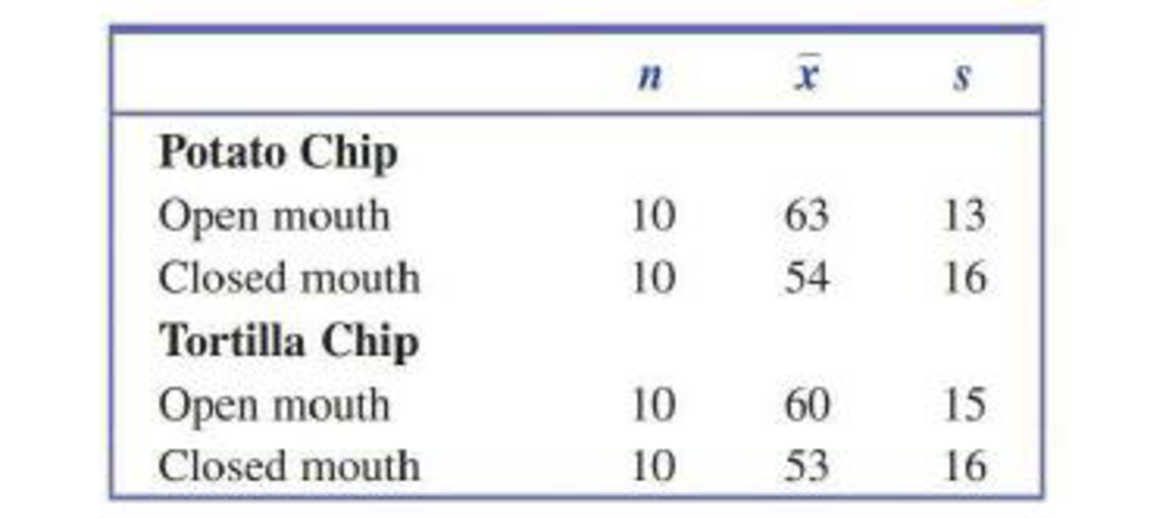
- a. Construct a 95% confidence interval tor the (inference in
mean peak loudness between open-mouth and closed-mouth chewing of potato chips. Interpret the resulting interval. - b. For closed-mouth chewing (the recommended method!), is there sufficient evidence to indicate that there is a difference between potato chips and tortilla chips with respect to mean peak loudness? Test the relevant hypotheses using α = 0.01.
- c. The means and standard deviations given here were actually for stale chips. When ten measurements of peak loudness were recorded for closed-mouth chewing of fresh tortilla chips, the resulting mean and standard deviation were 56 and 14, respectively. Is there sufficient evidence to conclude that chewing fresh tortilla chips is louder than chewing stale chips? Use α = 0.05.

Trending nowThis is a popular solution!

Chapter 11 Solutions
Introduction To Statistics And Data Analysis


- An article in the journal Air and Waste (Update on Ozone Trends in California's South Coast Air Basin, Vol. 43, 1993) investigated the ozone levels in the South Coast Air Basin of California for the years 1976-1991. The author believes that the number of days the ozone levels exceeded 0.20 ppm (the response) depends on the seasonal meteorological index, which is the seasonal average 850-millibar Temperature (the predictor). The following table gives the data. Year Index 1976 1977 1978 1979 1980 1981 1982 1983 1984 1985 1986 1987 1988 1989 1990 1991 Days 91 105 106 108 88 91 58 82 81 65 61 48 61 43 33 36 16.7 17.1 18.2 18.1 17.2 18.2 16.0 17.2 18.0 17.2 16.9 17.1 18.2 17.3 17.5 16.6 (a) Construct a scatter diagram of the data. (b) Estimate the prediction equation. (c) Test for significance of regression. (d) Calculate the 95% CI and PI on for a seasonal meteorological index value of 17. Interpret these quantities.arrow_forwardThe "spring-like effect" in a golf club could be determined by measuring the coefficient of restitution (the ratio of the outbound velocity to the inbound velocity of a golf ball fired at the clubhead). Twelve randomly selected drivers produced by two clubmakers are tested and the coefficient of restitution measured. The data follow: Club 1: 0.8406, 0.8104, 0.8234, 0.8198, 0.8235, 0.8562, 0.8123, 0.7976, 0.8184, 0.8265, 0.7773, 0.7871 Club 2: 0.8305, 0.7905, 0.8352, 0.8380, 0.8145, 0.8465, 0.8244, 0.8014, 0.8309, 0.8405, 0.8256, 0.8476 Test the hypothesis that both brands of ball have equal mean overall distance. Use α = 0.05 and assume equal variances. Question: Reject H0 if t0 < ___ or if t0 > ___.arrow_forwardAn education researcher claims that 60% of college students work year-round. In a random sample of 200 college students, 120 say they work year-round. At a = 0.10, is there enough evidence to reject the researcher's claim? Complete parts (a) through (e) below.arrow_forward
- An article in the ASCE Journal of Energy Engineering [“Overview of Reservoir Release Improvements at 20 TVA Dams” (Vol. 125, April 1999, pp. 1–17)] presents data on dissolved oxygen concentrations in streams below 20 dams in the Tennessee Valley Authority system. The observations are (in milligrams per liter):arrow_forwardHealth care workers who use latex gloves with glove powder on a daily basis are particularly susceptible to developing a latex allergy. Each in a sample of 44 hospital employees who were diagnosed with a latex allergy based on a skin-prick test reported on their exposure to latex gloves. Summary statistics for the number of latex gloves used per week are x= 19.4 and s = 11.7. Complete parts (a) - (d). a. Give a point estimate for the average number of latex gloves used per week by all health care workers with a latex allergy. b. Form a 95% confidence interval for the average number of latex gloves used per week by all health care workers with a latex allergy. (Use integers or decimals for any numbers in the expression. Round to two decimal places as needed.) c. Give a practical interpretation of the interval, part (b). O A. One can be 95% confident that latex gloves cause allergies for all who use a number of gloves contained in the interval. O B. One can be 95% confident that the…arrow_forwardA study was performed looking at the risk of fractures in three rural Iowa communities according to whether their drinking water was “higher calcium,” “higher fluorides,” or “control” as determined by water samples. Table 11.10 presents data comparing the rate of fractures (over 5 years) between the higher-calcium vs the control communities for women ages 20–35 and 55–80, respectively . Table 11.10 Relationship of calcium content of drinking water to the rate of fractures in rural Iowa Ages 20-35 Number of women with fractures Total number of women Ages 55-80 Number of woemn with fractures Total number of women Control 3 37 Control 11 121 High calcium 1 33 High calcium 21 148 13.1 What test can be used to compare the fracturerates in these two communities while controlling for age? 13.2 Implement the test in Problem 13.1, report a p-value, and make a conclusion on relationship between drinking water calcium concentration and rate of fracture based on the p-value.arrow_forward
- A study was performed looking at the risk of fractures in three rural Iowa communities according to whether their drinking water was “higher calcium,” “higher fluorides,” or “control” as determined by water samples. Table 11.10 presents data comparing the rate of fractures (over 5 years) between the higher-calcium vs the control communities for women ages 20–35 and 55–80, respectively . Table 11.10 Relationship of calcium content of drinking water to the rate of fractures in rural Iowa Ages 20-35 Number of women with fractures Total number of women Ages 55-80 Number of woemn with fractures Total number of women Control 3 37 Control 11 121 High calcium 1 33 High calcium 21 148 13.1 What test can be used to compare the fracturerates in these two communities while controlling for age? 13.2 Implement the test in Problem 13.1, report a p-value, and make a conclusion on relationship between drinking water calcium concentration and rate of fracture based on the p-value. 13.3…arrow_forwardA study of the relationship between age and various visual functions (such as acuity and depth perception) reported the following observations on the area of scleral lamina (mm2) from human optic nerve heads: 2.84 2.63 2.76 3.75 2.28 2.64 3.94 4.11 3.80 4.27 3.49 4.51 2.40 3.59 2.72 3.55 3.02 (a) Calculate Σxi and Σxi2. Σxi = ? mm2 Σxi2 = ? mm4 (b) Use the values calculated in part (a) to compute the sample variance s2 and then the sample standard deviation s. (Round your answers to four decimal places.) s2 = ? mm4 s = ? mm2arrow_forwardAn article in the Journal of Environmental Engineering (1989, Vol. 115(3), pp. 608–619) reported the results of a study on the occurrence of sodium and chloride in surface streams in central Rhode Island. The following data are chloride concentration y (in milligrams per liter) and roadway area in the watershed x (in percentage).arrow_forward
- In a study of exhaust emissions from school buses, the pollution intake by passengers was determined for a sample of nine school buses used in the Southern California Air Basin. The pollution intake is the amount of exhaust emissions, in grams per person, that would be inhaled while traveling on the bus during its usual 1818‑mile trip on congested freeways from South Central LA to a magnet school in West LA. (As a reference, the average intake of motor emissions of carbon monoxide in the LA area is estimated to be about 0.0000460.000046 grams per person.) The amounts for the nine buses when driven with the windows open are given. 1.151.15 0.330.33 0.400.40 0.330.33 1.351.35 0.380.38 0.250.25 0.400.40 0.350.35 A good way to judge the effect of outliers is to do your analysis twice, once with the outliers and a second time without them. Give two 90%90% confidence intervals, one with all the data and one with the outliers removed, for the mean pollution intake among all school buses…arrow_forwardHealth care workers who use latex gloves with glove powder on a daily basis are particularly susceptible to developing a latex allergy. Each in a sample of 47 hospital employees who were diagnosed with a latex allergy based on a skin-prick test reported on their exposure to latex gloves. Summary statistics for the number of latex gloves used per week are x = 19.7 and s = 12.1. Complete parts (a)-(d). a. Give a point estimate for the average number of latex gloves used per week by all health care workers with a latex allergy. 19.7 b. Form a 95% confidence interval for the average number of latex gloves used per week by all health care workers with a latex allergy. (16.24, 23.16) (Use integers or decimals for any numbers in the expression. Round to two decimal places as needed.) c. Give a practical interpretation of the interval, part (b). OA. One can be 95% confident that the average number of latex gloves used per week by all healthcare workers with latex allergy is greater than the…arrow_forwardThe toco toucan, the largest member of the toucan family, possesses the largest beak relative to body size of all birds. This exaggerated feature has received various interpretations, such as being a refined adaptation for feeding. However, the large surface area may also be an important mechanism for radiating heat (and hence cooling the bird) as outdoor temperature increases. The table contains data for beak heat loss, as a percentage of total body heat loss from all sources, at various temperatures in degrees Celsius. The data show that beak heat loss is higher at higher temperatures and that the relationship is roughly linear. [Note: The numerical values in this problem have been modified for testing purposes.] Temperature (Co) Percent heat loss from beak 15 32 16 34 17 35 18 33 19 37 20 46 21 55 22 51 23 43 24 52 25 45 26 53 27 58 28 60 29 62 30 62 Adapted from a graph in Glenn J. Tattersall et al., "Heat exchange from the toucan bill…arrow_forward
 Glencoe Algebra 1, Student Edition, 9780079039897...AlgebraISBN:9780079039897Author:CarterPublisher:McGraw Hill