Concept explainers
Videos
Compute the errors of bias and absolute deviation for the forecasts in problem 6 which of the
To compute: The errors of bias and absolute deviation and explain which forecast is the best.
Introduction:
Exponential smoothing:
In exponential smoothing forecast method, older data are given lesser importance, and newer data are given more importance. It is efficient in making short-term forecasts.
Explanation of Solution
Given information:
Forecast for period 1 (F1) = 90
Smoothing constant (α) = 0.1
| Period | Dt |
| 1 | 92 |
| 2 | 127 |
| 3 | 106 |
| 4 | 165 |
| 5 | 125 |
| 6 | 111 |
| 7 | 178 |
| 8 | 97 |
Formula for exponential smoothing:
Calculation of forecast:
The forecast for period 1 is 90.
Period 2:
The forecast for period 2 is 90.2.
Period 3:
The forecast for period 3 is 93.9.
Period 4:
The forecast for period 4 is 95.1.
Period 5:
The forecast for period 5 is 102.1.
Period 6:
The forecast for period 6 is 104.4.
Period 7:
The forecast for period 7 is 105.
Period 8:
The forecast for period 8 is 112.3.
Given information:
Forecast for period 1 (F1) = 90
Smoothing constant (α) = 0.3
| Period | Dt |
| 1 | 92 |
| 2 | 127 |
| 3 | 106 |
| 4 | 165 |
| 5 | 125 |
| 6 | 111 |
| 7 | 178 |
| 8 | 97 |
Calculation of forecast:
The forecast for period 1 is 90.
Period 2:
The forecast for period 2 is 90.6.
Period 3:
The forecast for period 3 is 101.5.
Period 4:
The forecast for period 4 is 102.9.
Period 5:
The forecast for period 5 is 121.5.
Period 6:
The forecast for period 6 is 122.6.
Period 7:
The forecast for period 7 is 119.1.
Period 8:
The forecast for period 8 is 136.8.
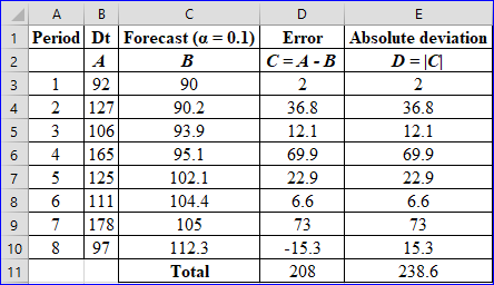
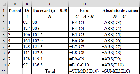
Calculation of error and absolute deviation:
For α = 0.1
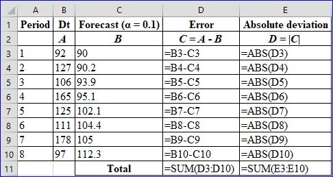
Excel work:
Excel formula:
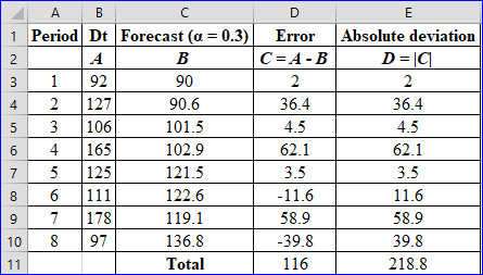
For α = 0.3
Excel work:
Excel formula:
For α = 0.1
Sum of error = 208
Sum of absolute deviation = 238.6
For α = 0.3
Sum of error = 116
Sum of absolute deviation = 218.8
The sum of error and absolute deviation is lower for α = 0.3 when compared with values of α = 0.1 (116 < 208) and (218.8 < 238.6). Hence, the forecasting method with α = 0.3 will be the best method.
The forecasting method with α = 0.3 is the best method.
Want to see more full solutions like this?
Chapter 10 Solutions
OPERATIONS MANAGEMENT IN THE SUPPLY CHAIN: DECISIONS & CASES (Mcgraw-hill Series Operations and Decision Sciences)


- The file P13_42.xlsx contains monthly data on consumer revolving credit (in millions of dollars) through credit unions. a. Use these data to forecast consumer revolving credit through credit unions for the next 12 months. Do it in two ways. First, fit an exponential trend to the series. Second, use Holts method with optimized smoothing constants. b. Which of these two methods appears to provide the best forecasts? Answer by comparing their MAPE values.arrow_forwardUnder what conditions might a firm use multiple forecasting methods?arrow_forwardThe owner of a restaurant in Bloomington, Indiana, has recorded sales data for the past 19 years. He has also recorded data on potentially relevant variables. The data are listed in the file P13_17.xlsx. a. Estimate a simple regression equation involving annual sales (the dependent variable) and the size of the population residing within 10 miles of the restaurant (the explanatory variable). Interpret R-square for this regression. b. Add another explanatory variableannual advertising expendituresto the regression equation in part a. Estimate and interpret this expanded equation. How does the R-square value for this multiple regression equation compare to that of the simple regression equation estimated in part a? Explain any difference between the two R-square values. How can you use the adjusted R-squares for a comparison of the two equations? c. Add one more explanatory variable to the multiple regression equation estimated in part b. In particular, estimate and interpret the coefficients of a multiple regression equation that includes the previous years advertising expenditure. How does the inclusion of this third explanatory variable affect the R-square, compared to the corresponding values for the equation of part b? Explain any changes in this value. What does the adjusted R-square for the new equation tell you?arrow_forward
- The Baker Company wants to develop a budget to predict how overhead costs vary with activity levels. Management is trying to decide whether direct labor hours (DLH) or units produced is the better measure of activity for the firm. Monthly data for the preceding 24 months appear in the file P13_40.xlsx. Use regression analysis to determine which measure, DLH or Units (or both), should be used for the budget. How would the regression equation be used to obtain the budget for the firms overhead costs?arrow_forwardThe file P13_29.xlsx contains monthly time series data for total U.S. retail sales of building materials (which includes retail sales of building materials, hardware and garden supply stores, and mobile home dealers). a. Is seasonality present in these data? If so, characterize the seasonality pattern. b. Use Winters method to forecast this series with smoothing constants = = 0.1 and = 0.3. Does the forecast series seem to track the seasonal pattern well? What are your forecasts for the next 12 months?arrow_forwardThe file P13_28.xlsx contains monthly retail sales of U.S. liquor stores. a. Is seasonality present in these data? If so, characterize the seasonality pattern. b. Use Winters method to forecast this series with smoothing constants = = 0.1 and = 0.3. Does the forecast series seem to track the seasonal pattern well? What are your forecasts for the next 12 months?arrow_forward
- The file P13_22.xlsx contains total monthly U.S. retail sales data. While holding out the final six months of observations for validation purposes, use the method of moving averages with a carefully chosen span to forecast U.S. retail sales in the next year. Comment on the performance of your model. What makes this time series more challenging to forecast?arrow_forwardThe file P13_02.xlsx contains five years of monthly data on sales (number of units sold) for a particular company. The company suspects that except for random noise, its sales are growing by a constant percentage each month and will continue to do so for at least the near future. a. Explain briefly whether the plot of the series visually supports the companys suspicion. b. By what percentage are sales increasing each month? c. What is the MAPE for the forecast model in part b? In words, what does it measure? Considering its magnitude, does the model seem to be doing a good job? d. In words, how does the model make forecasts for future months? Specifically, given the forecast value for the last month in the data set, what simple arithmetic could you use to obtain forecasts for the next few months?arrow_forwardThe file P13_26.xlsx contains the monthly number of airline tickets sold by the CareFree Travel Agency. a. Create a time series chart of the data. Based on what you see, which of the exponential smoothing models do you think will provide the best forecasting model? Why? b. Use simple exponential smoothing to forecast these data, using a smoothing constant of 0.1. c. Repeat part b, but search for the smoothing constant that makes RMSE as small as possible. Does it make much of an improvement over the model in part b?arrow_forward
- A small computer chip manufacturer wants to forecast monthly ozperating costs as a function of the number of units produced during a month. The company has collected the 16 months of data in the file P13_34.xlsx. a. Determine an equation that can be used to predict monthly production costs from units produced. Are there any outliers? b. How could the regression line obtained in part a be used to determine whether the company was efficient or inefficient during any particular month?arrow_forwardSuppose that a regional express delivery service company wants to estimate the cost of shipping a package (Y) as a function of cargo type, where cargo type includes the following possibilities: fragile, semifragile, and durable. Costs for 15 randomly chosen packages of approximately the same weight and same distance shipped, but of different cargo types, are provided in the file P13_16.xlsx. a. Estimate a regression equation using the given sample data, and interpret the estimated regression coefficients. b. According to the estimated regression equation, which cargo type is the most costly to ship? Which cargo type is the least costly to ship? c. How well does the estimated equation fit the given sample data? How might the fit be improved? d. Given the estimated regression equation, predict the cost of shipping a package with semifragile cargo.arrow_forwardThe file P13_25.xlsx contains the quarterly numbers of applications for home mortgage loans at a branch office of Northern Central Bank. a. Create a time series chart of the data. Based on what you see, which of the exponential smoothing models do you think will provide the best forecasting model? Why? b. Use simple exponential smoothing to forecast these data, using a smoothing constant of 0.1. c. Repeat part b, but search for the smoothing constant that makes RMSE as small as possible. Does it make much of an improvement over the model in part b? Is it guaranteed to produce better forecasts for the future?arrow_forward
 MarketingMarketingISBN:9780357033791Author:Pride, William MPublisher:South Western Educational Publishing
 Contemporary MarketingMarketingISBN:9780357033777Author:Louis E. Boone, David L. KurtzPublisher:Cengage Learning
 Practical Management ScienceOperations ManagementISBN:9781337406659Author:WINSTON, Wayne L.Publisher:Cengage,