
Videos
a.
State the null and alternate hypotheses.
a.
Answer to Problem 2CYU
The hypotheses are given below:
Null hypothesis:
That is, there is no significant difference between the
Alternate hypothesis:
That is, the mean amount of rainfall of the city in year2 is greater than the mean amount of rainfall of the city in year1.
Explanation of Solution
The data represents the mean amount of rainfall of a chosen city in two consecutive years (year2 and year1).
Hypothesis:
Hypothesis is an assumption about the parameter of the population, and the assumption may or may not be true.
Let
Claim:
Here, the claim is, whether the mean amount of rainfall of the city in year2 is greater than the mean amount of rainfall of the city in year1.
The hypotheses are given below:
Null hypothesis:
Null hypothesis is a statement which is tested for statistical significance in the test. The decision criterion indicates whether the null hypothesis will be rejected or not in the favor of alternate hypothesis.
That is, there is no significant difference between the mean amount of rainfall of a city in year2 and year1.
Alternate hypothesis:
Alternate hypothesis is contradictory statement of the null hypothesis
That is, the mean amount of rainfall of the city in year2 is greater than the mean amount of rainfall of the city in year1.
b.
Compute the differences in amount of rainfalls Year2– Year1.
b.
Answer to Problem 2CYU
The differences in amount of rainfalls Year2– Year1 is,
| S.no | |
| 1 | 9.5 |
| 2 | 3.4 |
| 3 | –3.8 |
| 4 | 10.1 |
| 5 | 8.9 |
| 6 | 5.7 |
Explanation of Solution
Calculation:
The differences in amount of rainfalls Year2– Year1 is,
| S.no | Year2 | Year1 | |
| 1 | 34.6 | 25.1 | |
| 2 | 18.7 | 15.3 | |
| 3 | 42.6 | 46.4 | |
| 4 | 41.3 | 31.2 | |
| 5 | 60.6 | 51.7 | |
| 6 | 29.9 | 24.2 |
c.
Find the value of t-test statistic.
c.
Answer to Problem 2CYU
The value of test statistic is 2.6118.
Explanation of Solution
Calculation:
Test statistic:
The test statistic for matched pairs is obtained as,
where
matched pairs and
Mean and standard deviation of differences:
Software procedure:
Step-by-step procedure to obtain the mean and standard deviation using the MINITAB software:
- Choose Stat > Basic statistic > Display
descriptive statistics . - In Variables, enter the column of Differences.
- In Statistics, select mean, standard deviation and N total.
- Click OK.
Output using the MINITAB software is given below:
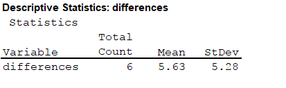
From the MINITAB output, the mean and standard deviation are 5.63 and 5.28.
The mean and standard deviation of the differences is 5.63 and 5.28.
Here, the
The test statistic is obtained as follows,
Thus, the test statistic is 2.6118.
d.
Find the P-value for the test statistic.
d.
Answer to Problem 2CYU
The P-value for the test statistic is 0.02378.
Explanation of Solution
Calculation:
Degrees of freedom:
The degrees of freedom for the test statistic is,
Thus, the degree of freedom is 5.
P-value:
Software procedure:
Step-by-step procedure to obtain the P-value using the MINITAB software:
- Choose Graph > Probability Distribution Plot.
- Choose View Probability > OK.
- From Distribution, choose ‘t’ distribution.
- In Degrees of freedom, enter 5.
- Click the Shaded Area tab.
- Choose X value and Right Tail for the region of the curve to shade.
- In X-value enter 2.6118.
- Click OK.
Output using the MINITAB software is given below:
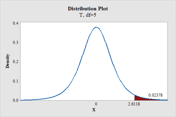
From the MINITAB output, the P-value is 0.02378.
Thus, the P-value is 0.02378.
e.
Interpret the P-value at the level of significance
e.
Answer to Problem 2CYU
There is enough evidence to reject the null hypothesis
Explanation of Solution
From part (d), the P-value is 0.02378.
Decision rule based on P-value:
If
If
Here, the level of significance is
Conclusion based on P-value approach:
The P-value is 0.02378 and
Here, P-value is less than the
That is,
By the rejection rule, reject the null hypothesis.
Thus, there is enough evidence to reject the null hypothesis
f.
State the conclusion.
f.
Answer to Problem 2CYU
There is enough evidence to conclude that the mean amount of rainfall of the city in year2 is greater than the mean amount of rainfall of the city in year1.
Explanation of Solution
From part (e), it is known that the null hypothesis is rejected.
That is, mean amount of rainfall of the city in year2 is greater than the mean amount of rainfall of the city in year1.
Thus, there is enough evidence to conclude that the mean amount of rainfall of the city in year2 is greater than the mean amount of rainfall of the city in year1.
Want to see more full solutions like this?
Chapter 9 Solutions
Essential Statistics


- Examine the Variables: Carefully review and note the names of all variables in the dataset. Examples of these variables include: Mileage (mpg) Number of Cylinders (cyl) Displacement (disp) Horsepower (hp) Research: Google to understand these variables. Statistical Analysis: Select mpg variable, and perform the following statistical tests. Once you are done with these tests using mpg variable, repeat the same with hp Mean Median First Quartile (Q1) Second Quartile (Q2) Third Quartile (Q3) Fourth Quartile (Q4) 10th Percentile 70th Percentile Skewness Kurtosis Document Your Results: In RStudio: Before running each statistical test, provide a heading in the format shown at the bottom. “# Mean of mileage – Your name’s command” In Microsoft Word: Once you've completed all tests, take a screenshot of your results in RStudio and paste it into a Microsoft Word document. Make sure that snapshots are very clear. You will need multiple snapshots. Also transfer these results to the…arrow_forwardExamine the Variables: Carefully review and note the names of all variables in the dataset. Examples of these variables include: Mileage (mpg) Number of Cylinders (cyl) Displacement (disp) Horsepower (hp) Research: Google to understand these variables. Statistical Analysis: Select mpg variable, and perform the following statistical tests. Once you are done with these tests using mpg variable, repeat the same with hp Mean Median First Quartile (Q1) Second Quartile (Q2) Third Quartile (Q3) Fourth Quartile (Q4) 10th Percentile 70th Percentile Skewness Kurtosis Document Your Results: In RStudio: Before running each statistical test, provide a heading in the format shown at the bottom. “# Mean of mileage – Your name’s command” In Microsoft Word: Once you've completed all tests, take a screenshot of your results in RStudio and paste it into a Microsoft Word document. Make sure that snapshots are very clear. You will need multiple snapshots. Also transfer these results to the…arrow_forwardExamine the Variables: Carefully review and note the names of all variables in the dataset. Examples of these variables include: Mileage (mpg) Number of Cylinders (cyl) Displacement (disp) Horsepower (hp) Research: Google to understand these variables. Statistical Analysis: Select mpg variable, and perform the following statistical tests. Once you are done with these tests using mpg variable, repeat the same with hp Mean Median First Quartile (Q1) Second Quartile (Q2) Third Quartile (Q3) Fourth Quartile (Q4) 10th Percentile 70th Percentile Skewness Kurtosis Document Your Results: In RStudio: Before running each statistical test, provide a heading in the format shown at the bottom. “# Mean of mileage – Your name’s command” In Microsoft Word: Once you've completed all tests, take a screenshot of your results in RStudio and paste it into a Microsoft Word document. Make sure that snapshots are very clear. You will need multiple snapshots. Also transfer these results to the…arrow_forward
- 2 (VaR and ES) Suppose X1 are independent. Prove that ~ Unif[-0.5, 0.5] and X2 VaRa (X1X2) < VaRa(X1) + VaRa (X2). ~ Unif[-0.5, 0.5]arrow_forward8 (Correlation and Diversification) Assume we have two stocks, A and B, show that a particular combination of the two stocks produce a risk-free portfolio when the correlation between the return of A and B is -1.arrow_forward9 (Portfolio allocation) Suppose R₁ and R2 are returns of 2 assets and with expected return and variance respectively r₁ and 72 and variance-covariance σ2, 0%½ and σ12. Find −∞ ≤ w ≤ ∞ such that the portfolio wR₁ + (1 - w) R₂ has the smallest risk.arrow_forward
- 7 (Multivariate random variable) Suppose X, €1, €2, €3 are IID N(0, 1) and Y2 Y₁ = 0.2 0.8X + €1, Y₂ = 0.3 +0.7X+ €2, Y3 = 0.2 + 0.9X + €3. = (In models like this, X is called the common factors of Y₁, Y₂, Y3.) Y = (Y1, Y2, Y3). (a) Find E(Y) and cov(Y). (b) What can you observe from cov(Y). Writearrow_forward1 (VaR and ES) Suppose X ~ f(x) with 1+x, if 0> x > −1 f(x) = 1−x if 1 x > 0 Find VaRo.05 (X) and ES0.05 (X).arrow_forwardJoy is making Christmas gifts. She has 6 1/12 feet of yarn and will need 4 1/4 to complete our project. How much yarn will she have left over compute this solution in two different ways arrow_forward
- Solve for X. Explain each step. 2^2x • 2^-4=8arrow_forwardOne hundred people were surveyed, and one question pertained to their educational background. The results of this question and their genders are given in the following table. Female (F) Male (F′) Total College degree (D) 30 20 50 No college degree (D′) 30 20 50 Total 60 40 100 If a person is selected at random from those surveyed, find the probability of each of the following events.1. The person is female or has a college degree. Answer: equation editor Equation Editor 2. The person is male or does not have a college degree. Answer: equation editor Equation Editor 3. The person is female or does not have a college degree.arrow_forwardneed help with part barrow_forward
 Glencoe Algebra 1, Student Edition, 9780079039897...AlgebraISBN:9780079039897Author:CarterPublisher:McGraw Hill