Chapter 9.3, Problem 10E

a.

To determine

Compute the differences in samples of matched pairs Sample-1– Sample-2.

Answer to Problem 10E

The differences in samples of matched pairs Sample-1– Sample-2 is,

S.no	Difference
1	–6
2	–1
3	–9
4	–1
5	–5
6	–1
7	–4
8	–8
9	–2
10	–9

Explanation of Solution

Calculation:

The data represents the sample of a five matched pairs.

Let ${\mu }_d={\mu }_1-{\mu }_2$ where ${\mu }_1$ be the population mean-1 is and ${\mu }_2$ be the population mean-2.

The differences in samples of matched pairs Sample-1– Sample-2 is,

S.no	Sample-1	Sample-2	$\text{Difference}\text{=}\text{Sample1}-\text{Sample2}$
1	28	34	$28-34=-6$
2	29	30	$29-30=-1$
3	22	31	$22-31=-9$
4	25	26	$25-26=-1$
5	26	31	$26-31=-5$
6	29	30	$29-30=-1$
7	27	31	$27-31=-4$
8	24	32	$24-32=-8$
9	27	29	$27-29=-2$
10	28	37	$28-37=-9$

b.

To determine

Find the value of t-test statistic.

Answer to Problem 10E

The value of test statistic is –4.3948.

Explanation of Solution

Calculation:

The test hypotheses are given below:

Null hypothesis:

$H_0:{\mu }_d=0$

That is, there is no significant difference between the population mean1 and population mean2.

Alternate hypothesis:

$H_1:{\mu }_d\ne 0$

That is, there is a significant difference between the population mean1 and population mean2.

Mean and standard deviation of differences:

Software procedure:

Step-by-step procedure to obtain the mean and standard deviation using the MINITAB software:

• Choose Stat > Basic statistic > Display descriptive statistics.
• In Variables, enter the column of Differences.
• In Statistics, select mean, standard deviation and N total.
• Click OK.

Output using the MINITAB software is given below:

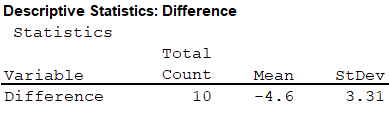
From the MINITAB output, the mean and standard deviation are –4.6 and 3.31.

The mean and standard deviation of the differences is –4.6 and 3.31.

The test statistic is obtained as follows,

$\begin{array}{c}t=\frac{\overline{d}-0}{\left(\frac{s_d}{\sqrt{n}}\right)}\\ =\frac{-4.6-0}{\left(\frac{3.31}{\sqrt{10}}\right)}\\ =\frac{-4.6}{1.0467}\\ =-4.3948\end{array}$

Thus, the test statistic is –4.3948.

c.

To determine

Check whether the null hypothesis is rejected at $\alpha =0.05$ level of significance.

Answer to Problem 10E

There is enough evidence to reject the null hypothesis $H_0$ at $\alpha =0.05$ level of significance.

Explanation of Solution

Degrees of freedom:

The degrees of freedom for the test statistic is,

$\begin{array}{c}d.f=n-1\\ =10-1\\ =9\end{array}$

Thus, the degree of freedom is 9.

P-value:

Software procedure:

Step-by-step procedure to obtain the P-value using the MINITAB software:

• Choose Graph > Probability Distribution Plot.
• Choose View Probability > OK.
• From Distribution, choose ‘t’ distribution.
• In Degrees of freedom, enter 9.
• Click the Shaded Area tab.
• Choose X value and Both Tail for the region of the curve to shade.
• In X-value enter –4.3948.
• Click OK.

Output using the MINITAB software is given below:

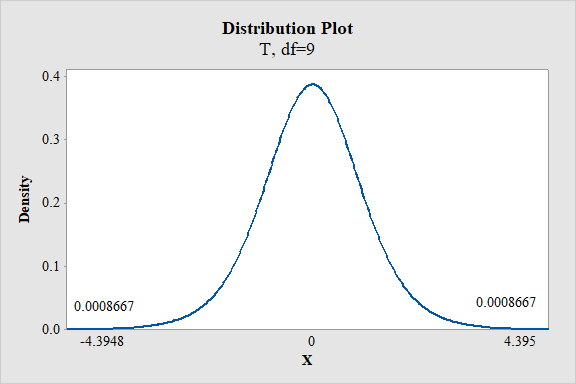
From the MINITAB output, the P-value is $2\times 0.0008667=0.0017$ .

Thus, the P-value is 0.0017.

Decision rule based on P-value:

If $P-\text{value}\le \alpha$, then reject the null hypothesis $H_0$.

If $P-\text{value}>\alpha$, then fail to reject the null hypothesis $H_0$.

Here, the level of significance is $\alpha =0.05$.

Conclusion based on P-value approach:

The P-value is 0.0017 and $\alpha$ value is 0.05.

Here, P-value is less than the $\alpha$ value.

That is, $0.0017\left(=P-\text{value}\right)<0.05\left(=\alpha \right)$.

By the rejection rule, reject the null hypothesis.

Thus, there is enough evidence to reject the null hypothesis $H_0$.

d.

To determine

Check whether the null hypothesis is rejected at $\alpha =0.01$ level of significance.

Answer to Problem 10E

There is enough evidence to reject the null hypothesis $H_0$ at $\alpha =0.01$ level of significance.

Explanation of Solution

From part (c), the P-value is 0.0017.

Decision rule based on P-value:

If $P-\text{value}\le \alpha$, then reject the null hypothesis $H_0$.

If $P-\text{value}>\alpha$, then fail to reject the null hypothesis $H_0$.

Here, the level of significance is $\alpha =0.01$.

Conclusion based on P-value approach:

The P-value is 0.0017 and $\alpha$ value is 0.01.

Here, P-value is less than the $\alpha$ value.

That is, $0.0017\left(=P-\text{value}\right)<0.01\left(=\alpha \right)$.

By the rejection rule, reject the null hypothesis.

Thus, there is enough evidence to reject the null hypothesis $H_0$.