Fluid Mechanics
8th Edition
ISBN: 9780073398273
Author: Frank M. White
Publisher: McGraw-Hill Education
expand_more
expand_more
format_list_bulleted
Videos
Textbook Question
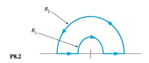
Chapter 8, Problem 8.2P
The steady plane flow in Fig. P8.2 has the polar velocity components
Expert Solution & Answer
Want to see the full answer?
Check out a sample textbook solution
Students have asked these similar questions
the flow of a stream
U, past a blunt flat plate creates a broad low-velocity wake
. , with
only half of the flow shown due to symmetry. The velocity
profile behind the plate is idealized as “dead air" (near-zero
velocity) behind the plate, plus a higher velocity, decaying
vertically above the wake according to the variation u =
U, + AU e2, where L is the plate height and z = 0 is the
top of the wake. Find AU as a function of stream speed Ug.
behind the plate. A simple model is given in Fig.
Uo
Exponential curve
Width b
Uo
into paper
U+AU
Dead air (negligible velocity)
€ -
Assume an inviscid, incompressible flow. Also, standard sea level density and pressure are 1.23 kg/m3 (0.002377 slug/ft3) and 1.01 × 10⁵ N/m2 (2116 lb/ft2), respectively.
Consider the lifting flow over a circular cylinder of a given radius and witha given circulation. If V∞ is doubled, keeping the circulation the same,does the shape of the streamlines change? Explain.
The flow past a two-dimensional Half-Rankine Body results from the superposition of a horizontal uniform flow of magnitude U= 3 m/s towards the right and a source of
strength g = 10 m2/s located at the origin (0, 0). The fluid density is 1000 kg/m³. All dimensional quantities are given in SI units. Neglect the effects of gravity.
The x-coordinate of the stagnation point is x =
m.
The total width of the body is
2.
m.
The magnitude of the pressure difference between the points (-1, 0) and (0, 2) is
kPa.
Enter the correct answer below.
Please enter a number for this text box.
2
Please enter a number for this text box.
Please enter a number for this text box.
Chapter 8 Solutions
Fluid Mechanics
Ch. 8 - Prob. 8.1PCh. 8 - The steady plane flow in Fig. P8.2 has the polar...Ch. 8 - P8.3 Using cartesian coordinates, show that each...Ch. 8 - P8.4 Is the function 1/r a legitimate velocity...Ch. 8 - Prob. 8.5PCh. 8 - An incompressible plane flow has the velocity...Ch. 8 - Prob. 8.7PCh. 8 - For the velocity distribution u=By,=+Bx , evaluate...Ch. 8 - Prob. 8.9PCh. 8 - Prob. 8.10P
Ch. 8 - Prob. 8.11PCh. 8 - Prob. 8.12PCh. 8 - P8.13 Starting at the stagnation point in Fig....Ch. 8 - P8.14 A tornado may be modeled as the circulating...Ch. 8 - Hurricane Sandy, which hit the New Jersey coast on...Ch. 8 - Prob. 8.16PCh. 8 - P8.17 Find the position (x, y) on the upper...Ch. 8 - Prob. 8.18PCh. 8 - Prob. 8.19PCh. 8 - Plot the streamlines of the flow due to a line...Ch. 8 - P8.21 At point A in Fig. P8.21 is a clockwise line...Ch. 8 - P8.22 Consider inviscid stagnation flow, (see...Ch. 8 - P8.23 Sources of strength m = 10 m2/s are placed...Ch. 8 - P8.24 Line sources of equal strength m = Ua, where...Ch. 8 - Prob. 8.25PCh. 8 - Prob. 8.26PCh. 8 - Prob. 8.27PCh. 8 - Sources of equal strength m are placed at the four...Ch. 8 - Prob. 8.29PCh. 8 - Prob. 8.30PCh. 8 - A Rankine half-body is formed as shown in Fig....Ch. 8 - Prob. 8.32PCh. 8 - P8.33 Sketch the streamlines, especially the body...Ch. 8 - Prob. 8.34PCh. 8 - Prob. 8.35PCh. 8 - Prob. 8.36PCh. 8 - Prob. 8.37PCh. 8 - Consider potential flow of a uniform stream in the...Ch. 8 - A large Rankine oval, with a = 1 m and h = 1 m, is...Ch. 8 - Prob. 8.40PCh. 8 - Prob. 8.41PCh. 8 - Prob. 8.42PCh. 8 - P8.43 Water at 20°C flows past a 1-rn-diameter...Ch. 8 - Prob. 8.44PCh. 8 - Prob. 8.45PCh. 8 - P8.46 A cylinder is formed by bolting two...Ch. 8 - Prob. 8.47PCh. 8 - Prob. 8.48PCh. 8 - Prob. 8.49PCh. 8 - It is desired to simulate flow past a...Ch. 8 - Prob. 8.51PCh. 8 -
P8.52 The Flettner rotor sailboat in Fig. E8.3...Ch. 8 - P8.52 The Flettner rotor sailboat in Fig. E8.3 has...Ch. 8 - Prob. 8.54PCh. 8 - Prob. 8.55PCh. 8 - Prob. 8.56PCh. 8 - Prob. 8.57PCh. 8 - Prob. 8.58PCh. 8 - Prob. 8.59PCh. 8 - Prob. 8.60PCh. 8 - Prob. 8.61PCh. 8 - Prob. 8.62PCh. 8 - The superposition in Prob. P8.62 leads to...Ch. 8 - Consider the polar-coordinate stream function...Ch. 8 - Prob. 8.65PCh. 8 - Prob. 8.66PCh. 8 - Prob. 8.67PCh. 8 - Prob. 8.68PCh. 8 - Prob. 8.69PCh. 8 - Prob. 8.70PCh. 8 - Prob. 8.71PCh. 8 - Prob. 8.72PCh. 8 - Prob. 8.73PCh. 8 - Prob. 8.74PCh. 8 - Prob. 8.75PCh. 8 - Prob. 8.76PCh. 8 - Prob. 8.77PCh. 8 - Prob. 8.78PCh. 8 - Prob. 8.79PCh. 8 - Prob. 8.80PCh. 8 - Prob. 8.81PCh. 8 - Prob. 8.82PCh. 8 - Prob. 8.83PCh. 8 - Prob. 8.84PCh. 8 - Prob. 8.85PCh. 8 - Prob. 8.86PCh. 8 - Prob. 8.87PCh. 8 - Prob. 8.88PCh. 8 - Prob. 8.89PCh. 8 - NASA is developing a swing-wing airplane called...Ch. 8 - Prob. 8.91PCh. 8 - Prob. 8.92PCh. 8 - Prob. 8.93PCh. 8 - Prob. 8.94PCh. 8 - Prob. 8.95PCh. 8 - Prob. 8.96PCh. 8 - Prob. 8.97PCh. 8 - Prob. 8.98PCh. 8 - Prob. 8.99PCh. 8 - Prob. 8.100PCh. 8 - Prob. 8.101PCh. 8 - Prob. 8.102PCh. 8 - Prob. 8.103PCh. 8 - Prob. 8.104PCh. 8 - Prob. 8.105PCh. 8 - Prob. 8.106PCh. 8 - Prob. 8.107PCh. 8 - P8.108 Consider two-dimensional potential flow...Ch. 8 - Prob. 8.109PCh. 8 - Prob. 8.110PCh. 8 - Prob. 8.111PCh. 8 - Prob. 8.112PCh. 8 - Prob. 8.113PCh. 8 - Prob. 8.114PCh. 8 - Prob. 8.115PCh. 8 - Prob. 8.1WPCh. 8 - Prob. 8.2WPCh. 8 - Prob. 8.3WPCh. 8 - Prob. 8.4WPCh. 8 - Prob. 8.5WPCh. 8 - Prob. 8.6WPCh. 8 - Prob. 8.7WPCh. 8 - Prob. 8.1CPCh. 8 - Prob. 8.2CPCh. 8 - Prob. 8.3CPCh. 8 - Prob. 8.4CPCh. 8 - Prob. 8.5CPCh. 8 - Prob. 8.6CPCh. 8 - Prob. 8.7CPCh. 8 - Prob. 8.1DPCh. 8 - Prob. 8.2DPCh. 8 - Prob. 8.3DP
Knowledge Booster


Learn more about
Need a deep-dive on the concept behind this application? Look no further. Learn more about this topic, mechanical-engineering and related others by exploring similar questions and additional content below.Similar questions
- Problem 6: Consider the incompressible Newtonian pipe flow (Fig. 6). Assume the flow is essentially axial, vz + 0 but v = ve = 0 and ôlƏe = 0. The flow is fully developed and steady in a horizontal pipe with the constant pressure gradient. Apply the Navier-Stokes equations and: a) Develop simplified governing equations (continuity and momentum) for this flow; b) Apply the boundary conditions and determine the velocity profile; and c) Develop expressions for the flow rate and mean velocity from the velocity profile. Vz Fig. 6 Flow in circular pipe 1.1 GB used DELL F5 F6 F7 F8 211arrow_forwardOne of the corner flow patterns of Fig. 8.18 is given by thecartesian stream function ψ = A(3yx2 - y3). Which one?Can the correspondence be proved ?arrow_forwardFrom the laminar boundary layer the velocity distributions given below, find the momentum thickness θ, boundary layer thickness δ, wall shear stress τw, skin friction coefficient Cf , and displacement thickness δ*1. A linear profile, u(x, y) = a + by 2. von K ́arm ́an’s second-order, parabolic profile,u(x, y) = a + by + cy2 3. A third-order, cubic function,u(x, y) = a + by + cy2+ dy3 4. Pohlhausen’s fourth-order, quartic profile,u(x, y) = a + by + cy2+ dy3+ ey4 5. A sinusoidal profile,u = U sin (π/2*y/δ)arrow_forward
- A tornado may be modeled as the circulating flow shown in Fig. : , with v, = v, = (0 and v(r) such that wr rsR Vg = {wR r> R Determine whether this flow pattern is irotational in either the inner or outer region. Using the r-momentum equation (D.5) of App. D, determine the pressure distribution p(r) in the tornado, assuming p = po as r→ o. Find the location and magnitude of the lowest pressure. (r) -rarrow_forwardQ.3Given the x and y velocity components below (A is a constant): u = Axt v = -Ayt (a) Find the equation of the streamlines, also give the stream function. (b) Find the equation of the streamline passing from x = 2 m and y = 3 m.arrow_forwardTwo free vortices of equal strength. but opposite direction of rotation, are superimposed with a uniform flow as shown in Fig. 4 1. The stream functions for these two vorticies are V = -[±T/2#)] In r. (a) Develop an equation for the x-component of velocity, u, at point P(x,y) in terms of Cartesian coordinates x and y. (b) Compute the x-component of velocity at point A and show that it depends on the ratio I'/H. 4- Sketch and describe the flow then determine the stagnation points. •Plx, y) Figure (4)arrow_forward
- 1. For a certain incompressible two-dimensional flow, the stream function, ψ(x, y) is prescribed. Is the continuity equation satisfied? 2. If u = −Ae−ky cos kx and v = −Ae−ky sin kx, find the stream function. Is this flow rotational, or irrotational?arrow_forwardConsider steady flow of water through an axisymmetric garden hose nozzle. Along the centerline of the nozzle, the water speed increases from uentrance to uexit as sketched. Measurements reveal that the centerline water speed increases parabolically through the nozzle. Write an equation for centerline speed u(x), based on the parameters given here, from x = 0 to x = Larrow_forwardConsider steady flow of water through an axisymmetric garden hose nozzle. Along the centerline of the nozzle, the water speed increases from uentrance to uexit as sketched. Measurements reveal that the centerline water speed increases parabolically through the nozzle, calculate the fluid acceleration along the nozzle centerline as a function of x and the given parameters.arrow_forward
- ASAParrow_forwardQ.5 The velocity components in x and y direction 2 are given by u = Axy° - xy; v = > ху; v — ху = xy² – 3/4 .4 y*. The value of A for a possible flow field involving an incompressible fluid is: A -3/4 В 3 C 4/3 D -4/3arrow_forwardA solid cone of angle 2Ɵ, base r 0 , and density ρ c is rotating with initialangular velocity ω 0 inside a conical seat,as shown below. The clearance h is filled with oilof viscosity μ. Neglecting air drag, derive an analytical expression for thecone’s angular velocity ω(t) if there is noapplied torque.arrow_forward
arrow_back_ios
SEE MORE QUESTIONS
arrow_forward_ios
Recommended textbooks for you
 Elements Of ElectromagneticsMechanical EngineeringISBN:9780190698614Author:Sadiku, Matthew N. O.Publisher:Oxford University Press
 Mechanics of Materials (10th Edition)Mechanical EngineeringISBN:9780134319650Author:Russell C. HibbelerPublisher:PEARSON
 Thermodynamics: An Engineering ApproachMechanical EngineeringISBN:9781259822674Author:Yunus A. Cengel Dr., Michael A. BolesPublisher:McGraw-Hill Education
 Control Systems EngineeringMechanical EngineeringISBN:9781118170519Author:Norman S. NisePublisher:WILEY
 Mechanics of Materials (MindTap Course List)Mechanical EngineeringISBN:9781337093347Author:Barry J. Goodno, James M. GerePublisher:Cengage Learning
 Engineering Mechanics: StaticsMechanical EngineeringISBN:9781118807330Author:James L. Meriam, L. G. Kraige, J. N. BoltonPublisher:WILEY
Elements Of Electromagnetics
Mechanical Engineering
ISBN:9780190698614
Author:Sadiku, Matthew N. O.
Publisher:Oxford University Press
Mechanics of Materials (10th Edition)
Mechanical Engineering
ISBN:9780134319650
Author:Russell C. Hibbeler
Publisher:PEARSON
Thermodynamics: An Engineering Approach
Mechanical Engineering
ISBN:9781259822674
Author:Yunus A. Cengel Dr., Michael A. Boles
Publisher:McGraw-Hill Education
Control Systems Engineering
Mechanical Engineering
ISBN:9781118170519
Author:Norman S. Nise
Publisher:WILEY
Mechanics of Materials (MindTap Course List)
Mechanical Engineering
ISBN:9781337093347
Author:Barry J. Goodno, James M. Gere
Publisher:Cengage Learning
Engineering Mechanics: Statics
Mechanical Engineering
ISBN:9781118807330
Author:James L. Meriam, L. G. Kraige, J. N. Bolton
Publisher:WILEY
Intro to Compressible Flows — Lesson 1; Author: Ansys Learning;https://www.youtube.com/watch?v=OgR6j8TzA5Y;License: Standard Youtube License