
a.
To calculate: The linear regression models and superimpose its graph on a
The obtained matrix is
Given Information:
The table is defined,
| Time (years) | Disbursements (billions of $) |
| 2005 | 336.9 |
| 2010 | 521.2 |
| 2011 | 560.3 |
| 2012 | 550.1 |
| 2013 | 581.7 |
| 2014 | 600.3 |
| 2015 | 638.1 |
Calculation:
Consider the given table,
| Time (years) | Disbursements (billions of $) |
| 2005 | 336.9 |
| 2010 | 521.2 |
| 2011 | 560.3 |
| 2012 | 550.1 |
| 2013 | 581.7 |
| 2014 | 600.3 |
| 2015 | 638.1 |
Use a graphing calculator to find the linear rgeression.
Step 1. Insert the table in calculator by using the table feature.
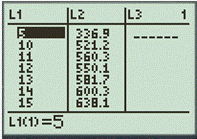
Step 2. Use the LinReg feature with first two list
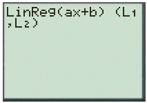
And,
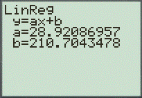
Step 3. Use the Graph feature to plot the both the graph as scatter graph.
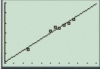
Therefore, the obtained equation is
b.
To calculate: The logistic regression model and superimpose its graph on a scatter plot of the data.
The obtained model is
Given Information:
The table is defined,
| Time (years) | Disbursements (billions of $) |
| 2005 | 336.9 |
| 2010 | 521.2 |
| 2011 | 560.3 |
| 2012 | 550.1 |
| 2013 | 581.7 |
| 2014 | 600.3 |
| 2015 | 638.1 |
Calculation:
Consider the given table,
| Time (years) | Disbursements (billions of $) |
| 2005 | 336.9 |
| 2010 | 521.2 |
| 2011 | 560.3 |
| 2012 | 550.1 |
| 2013 | 581.7 |
| 2014 | 600.3 |
| 2015 | 638.1 |
Use a graphing calculator to find the logestic model.
Step 1. Insert the table in calculator by using the table feature.
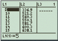
Step 2. Use the LinReg feature with first two list
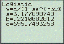
Step 3. Use the Graph feature to plot the both the graph as scatter graph.
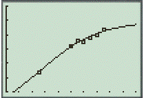
Hence, the obtained result is
c.
To determine: The models in parts (a) and (b) predict the same disbursement amounts.
The obtained model is
Given Information:
The table is defined,
| Time (years) | Disbursements (billions of $) |
| 2005 | 336.9 |
| 2010 | 521.2 |
| 2011 | 560.3 |
| 2012 | 550.1 |
| 2013 | 581.7 |
| 2014 | 600.3 |
| 2015 | 638.1 |
Calculation:
Consider the given table,
| Time (years) | Disbursements (billions of $) |
| 2005 | 336.9 |
| 2010 | 521.2 |
| 2011 | 560.3 |
| 2012 | 550.1 |
| 2013 | 581.7 |
| 2014 | 600.3 |
| 2015 | 638.1 |
Use a graphing calculator to find the logestic model.
Step 1. Insert the table in calculator by using the table feature.
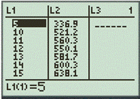
Step 2. Graph the both equations (a) and (b) then use the intersect feature to find the intersection point.
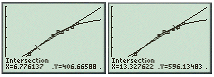
The x -coordinates are about 6.8 and 13.3, representing the years 2006 and 2013, respectively.
Hence, the obtained years are 2006 and 2013.
d.
To determine: The models, which appears to be a better fit for the data and explain which model would you choose to make predictions beyond 2020
The first choice is logistic model and then linear model.
Given Information:
The table is defined,
| Time (years) | Disbursements (billions of $) |
| 2005 | 336.9 |
| 2010 | 521.2 |
| 2011 | 560.3 |
| 2012 | 550.1 |
| 2013 | 581.7 |
| 2014 | 600.3 |
| 2015 | 638.1 |
Calculation:
Consider the given information,
The logistic model seems to be a better fit for the data since it passes most points compared to the linear model. For predictions beyond 2020, I would choose the linear model because the trend of the disbursement appears to be increasing.
The logistic model has a limiting growth of about 696 billion dollars which does not make sense in real life.
Hence, the first choice is logistic model and then linear model.
Chapter 7 Solutions
PRECALCULUS:GRAPHICAL,...-NASTA ED.
 Calculus: Early TranscendentalsCalculusISBN:9781285741550Author:James StewartPublisher:Cengage Learning
 Thomas' Calculus (14th Edition)CalculusISBN:9780134438986Author:Joel R. Hass, Christopher E. Heil, Maurice D. WeirPublisher:PEARSON
 Calculus: Early Transcendentals (3rd Edition)CalculusISBN:9780134763644Author:William L. Briggs, Lyle Cochran, Bernard Gillett, Eric SchulzPublisher:PEARSON
 Calculus: Early TranscendentalsCalculusISBN:9781319050740Author:Jon Rogawski, Colin Adams, Robert FranzosaPublisher:W. H. Freeman
 Calculus: Early Transcendental FunctionsCalculusISBN:9781337552516Author:Ron Larson, Bruce H. EdwardsPublisher:Cengage Learning


