
(a)
Estimated regression line.
(a)
Explanation of Solution
The formula for the regression equation is:
Run the ordinary least squares method for the given data in excel. The results drawn are as follows:
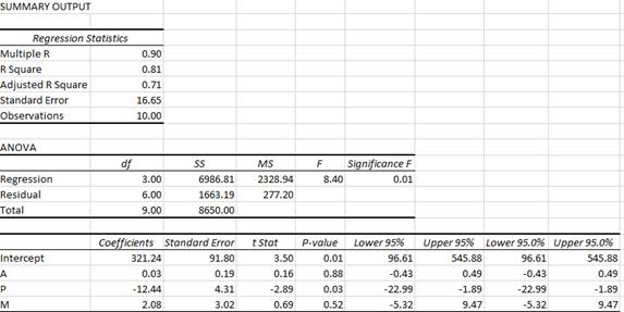
Use the summary output to find the estimated regression equation as follows:
(b)
The economic interpretation of the estimated intercept (a) and slope (b) coefficients.
(b)
Explanation of Solution
Interpretation of estimated intercept (a) coefficient:
When the selling price, promotional expenditure and disposable income are zero, on average the quantity sold of pens is equal to 321.24× $1000 = $321,240.
Interpretation of estimated slope (b) coefficient:
For a given level of selling price and disposable income, an additional $1,000 promotional expenditures lead to a rise in sales by 0.03×1000 = 30 gallons on average.
For a given level of promotional expenditure and selling price, an additional $1,000 disposable income leads to a rise in sales by 2.08×1000 = 2,080 gallons on an average.
For a given level of promotional expenditure and disposable income, an additional $1/gallon lead to falling in sales by 12.44×1000 = 12,440 gallons on an average.
(c)
The hypothesis that there is no relationship between the variables at 0.05 significance level.
(c)
Explanation of Solution
Conduct the t-test to know the statistical significance of the independent variables A, Pand M. The test statistic can be calculated using the following formula:
The t-statistic follows t-distribution with n-1 degrees of freedom.
For variable A, t-test is conducted as follows:
According to the summary output, the t-statistic for A variable is equal to 0.16.
At 5% significance level and 10-1=9 degrees of freedom, the critical value is equal to 2.262.
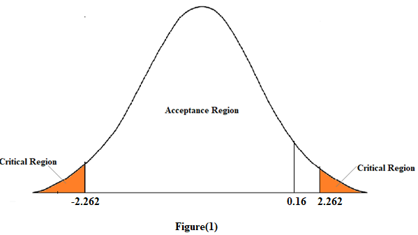
In figure (1), since the calculated t-statistic lies in the acceptance region. Therefore, we accept the null hypothesis. This means that the variable A is not statistically significant.
For variable P, t-test is conducted as follows:
According to the summary output, the t-statistic for P variable is equal to -2.89. At 5% significance level and 10-1=9 degrees of freedom, the critical value is equal to 2.262.
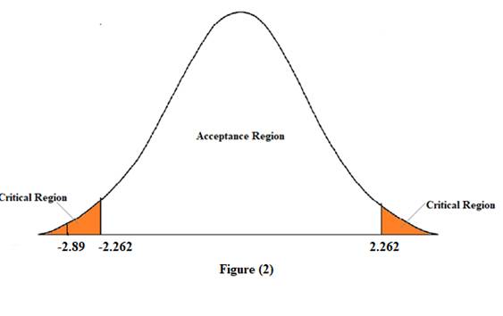
In figure (2), since the calculated t-statistic lies in the critical region. Therefore, we reject the null hypothesis. This means that the variable Pis statistically significant.
For variable M, t-test is conducted as follows:
According to the summary output, the t-statistic for M variable is equal to 0.69.
At 5% significance level and 10-1=9 degrees of freedom, the critical value is equal to 2.262.
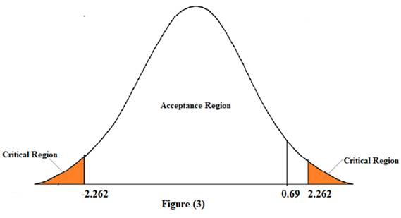
In figure (3), since the calculated t-statistic lies in the acceptance region. Therefore, we accept the null hypothesis. This means that the M variable is not statistically significant.
(d)
Coefficient of determination.
(d)
Explanation of Solution
The coefficient of determination measures the proportion of variance predicted by the independent variable in the dependent variable. It is denoted as R2.
According to the summary output, the value of R2 is equal to 0.81. This means that the regression equation predicts 81% of the variance in sales.
(e)
(e)
Explanation of Solution
The value of F-statistic is given as 8.40. And the critical value at 0.05 significance level is equal to 0.01.
Since F-statistic is greater than the critical value, thus, the overall model is statistically significant.
(f)
Best estimate of the product sales when the selling price is $14.50. And an approximate 95 percent prediction interval.
(f)
Explanation of Solution
According to the regression statistics of the summary output, for a given level of promotional expenditure and disposable income, $14.50/gallon lead to fall in sales by 12.44×14.50×1000 = 180,380 gallons on an average.
According to the regression statistics in the summary output, a 95% confidence interval for the P variable ranges from -22.99 to -1.89.
(g)
Price elasticity of demand at a selling price of $14.50.
(g)
Explanation of Solution
Formula to calculate elasticity in linear regression model is as follows:
At given value of P variable equal to 14.50, the estimated value of Y variable is equal to 180,380.
Thus, price elasticity of demand is calculated as follows:
Thus, the price elasticity of demand at a selling price of $14.50 is equal to -0.001.
Want to see more full solutions like this?
Chapter 4 Solutions
Managerial Economics: Applications, Strategies and Tactics (MindTap Course List)

- Suppose you decide to estimate a student consumption function. After you run an OLS regression on your data set with 36 observations, you obtain the following. The estimated regression, along with standard errors and t-statistics, CO = - 47.143 + 0.9714 YD (se) (2.0307) (0.157) (t) ( ) (6.187) Where, CO : the average annual consumption expenditures of the students on items other than tuition and room. YD : the average annual disposable income (including gifts) of the students Suppose that disposable income is increased by 1000 dollars on average. What would be the predicted consumption expenditures?arrow_forward2. Consider a two variable regression model, which satisfies all the Gauss Markov assumptions except that the error variance is proportional to X² i.e.E(u?) = o²X? Y₁ = B₁ + B₂X₁ + Ui How would you obtain the best linear unbiased estimates from the above regression.arrow_forwardConsider a data set with 15 observations and consider a multiple linear regression model with 7 in-dependent variables. Assume you have estimated the model and you find that SST = 1,325 and SSR = 794.arrow_forward
- Consider the polynomial regression model Yį = ßo + B₁X; + ß₂X² + uį, which of the following is true? This is a second-degree polynomial regression model This is a simple regression model because there is only one explanatory variable OLS is problematic in estimating the parameters due to the multicollinearity problem All the parameters (B's) must have the same signarrow_forward1. Data were collected on sales of mountain bikes in 30 sporting goods stores. The regression model was y = total sales (thousands of dollars), *₁ = display floor space (square meters), 2 = competitors' advertising expenditures (thousands of dollars), and x3 = advertised price (dollars per unit). A summary of the regression output is below. Variable (nickname) Intercept FloorSpace Competing Ads Price Coefficient 1225.44 11.52 -6.935 -0.1496 (a) Write the fitted regression equation. Round your coefficient Competing Ads to 3 decimal places, coefficient Price to 4 decimal places, and other values to 2 decimal places. (b-1) Put an X in the correct answer circle. The coefficient of FloorSpace says that each additional square foot of floor space... O adds about 11.52 to sales (in thousands of dollars). takes away 11.52 from sales (in thousands of dollars). O adds about 6.935 to sales (in thousands of dollars). takes away 0.1496 from sales (in thousands of dollars). (b-2) Put an X in the…arrow_forwardConsider the following regression model and corresponding output for a dataset with n = 104 observations: y=ß₁+ß2x2+ß³¸*¸+4 3 4x4+u Variable β Std. Error t P>|t| X2 -0.012 0.006 -2.289 0.022 X3 0.596 0.014 41.139 0.000 X4 0.52 1.06 Constant 8.860 1.766 5.017 0.000 What is the marginal effect of x4 on y? (approximate at least to 3 decimal places)arrow_forward
- An economist believes that price, x, (in dollars) is the biggest factor affecting quantity sold, y. To support his argument, he collected data on price and quantity sold from a sample of 29 stores, selling the same product, and generated the regression output in Excel. The regression equation is reported as y = and the correlation coefficient r = - 0.333. 9.45x + 20.86 What proportion of the variation in quantity sold y can be explained by the variation in price? R² = % Report answer as a percentage accurate to one decimal place.arrow_forwardY-1.04 +0.24X₁-0.27X2 where Y = quarterly sales (in thousands of cases) of the cold remedy X₁ = Cascade's quarterly advertising (x $1,000) for the cold remedy X₂= competitors' advertising for similar products (x $10,000) Here is additional information concerning the regression model: 8b1 = 0.052, 862 = 0.080, R² = 0.640, 8e-1.63, F-statistic=31.402, and Durbin-Watson (d) statistic=0.499. Which of the independent variables (if any) appears to be statistically significant (at the 0.05 level) in explaining sales of the remedy? (Hint: to.05/2,33-32.042.) Check all that apply. □ X₁ OX2 What proportion of the total variation in sales is explained by the regression equation? 0.640 0.080 O 0.132 O 0.052 The given F-value shows that you reject the null hypothesis that neither of the independent variables explains a significant (at the 0.05 level) proportion of the variation in income. (Hint: Fo.05,2,33-2-F3.316.)arrow_forwardA. B. Consider data on births to women in the United States. Two variables of interest are the dependent variable, infant birth weight in ounces (bwght), and an explanatory variable, average number of cigarettes the mother smoked per day during pregnancy (cigs). The following simple regression was estimated using data on n = 1,388 births: bwght = 119.772 (0.572) n = 1,388, 0.514 cigs (0.091) R² = 0.0227, where standard errors are shown in parenthesis. What percent of the variation in birth weight is explained by cigs? What is the predicted birth weight when cigs = 0? What about when cigs = 20 (one pack per day)? Comment on the difference.arrow_forward
- Find the degrees of freedom in a regression model that has 10 observations and 7 independent variablesarrow_forwardSuppose there are 2 quantitative free variables and 1 variable non free category. Non-free variables have 2 categories, namely 1 for the success category and 1 for the fail category. The method used to create models that describe relationships between variables is a binary logistic regression model. Perform parameter recovery for the model. Explain the stage until the alleged value is obtainedarrow_forwardThe best way to interpret polynomial regressions is to: A. look at the t-statistics for the relevant coefficients. B. analyze the standard error of estimated effect. C. plot the estimated regression function and to calculate the estimated effect on Y associated with a change in X for one or more values of X. D. take a derivative of Y with respect to the relevant X.arrow_forward
 Managerial Economics: Applications, Strategies an...EconomicsISBN:9781305506381Author:James R. McGuigan, R. Charles Moyer, Frederick H.deB. HarrisPublisher:Cengage Learning