An Introduction to Statistical Methods and Data Analysis
7th Edition
ISBN: 9781305269477
Author: R. Lyman Ott, Micheal T. Longnecker
Publisher: Cengage Learning
expand_more
expand_more
format_list_bulleted
Videos
Textbook Question
Chapter 3.11, Problem 32E
Many marine phanerogam species are highly sensitive to changes in environmental conditions. In the article “Posidonia oceanica: A Biological Indicator of Past and Present Mercury Contamination in the Mediterranean Sea’’ [Marine Environmental Research, March 1998 45:101–111], the researchers report the mercury concentrations over a period of about 20 years at several locations in the Mediterranean Sea. Samples of Posidonia oceanica were collected by scuba diving at a depth of 10 meters. For each site, 45 orthotropic shoots were sampled and the mercury concentration was determined. The average mercury concentration is recorded in the following table for each of the sampled years.
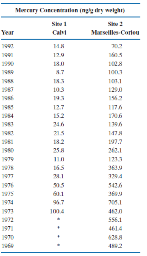
- a. Generate a time-series plot of the mercury concentrations and place lines for both sites on the same graph. Comment on any trends in the lines across the years of data. Are the trends similar for both sites?
- b. Select the most appropriate measure of center for the mercury concentrations. Compare the centers for the two sites.
- c. Compare the variabilities of the mercury concentrations at the two sites. Use the CV in your comparison, and explain why it is more appropriate than using the standard deviations.
- d. When comparing the centers and variabilities of the two sites, should the years 1969–1972 be used for site 2?
Expert Solution & Answer
Want to see the full answer?
Check out a sample textbook solution
Students have asked these similar questions
Cheek teeth of extinct primates. The characteristics of cheek teeth (e.g., molars) can provide anthropologists with information on the dietary habits of extinct mammals. The cheek teeth of an extinct primate species were the subject of research reported in the American Journal of Physical Anthropology (Vol. 142, 2010). A total of 18 cheek teeth extracted from skulls discovered in western Wyoming were analyzed. Researchers recorded the dentary depth of molars (in millimeters) for a sample of 18 cheek teeth extracted from skulls. These depth measurements are listed in the accompanying table. Anthropologists know that the mean dentary depth of molars in an extinct primate species— called Species A—is 15 millimeters. Is there evidence to indicate that the sample of 18 cheek teeth come from some other extinct primate species (i.e., some species other than Species A)?
The data are given below (you will need to put it into a single column). You will need to calculate the sample…
An article in the ASCE Journal of Energy Engineering [“Overview of Reservoir Release Improvements at 20 TVA Dams” (Vol. 125, April 1999, pp. 1–17)] presents data on dissolved oxygen concentrations in streams below 20 dams in the Tennessee Valley Authority system. The observations are (in milligrams per liter):
The article "Characteristics and Trends of River Discharge into Hudson, James, and Ungava
Bays, 1964-2000" (S. Dery, M. Stieglitz, et al., Journal of Climate, 2005:2540-2557)
presents measurements of discharge rate x (in kmlyr) andpeakflow y (in m/s) for 42 rivers
that drain into the Hudson, James, and Ungava Bays. The data are shown in the following
table:
Discharge
Peak Flow
94.24
4110.3
66.57
4961.7
59.79
10275.5
48.52
6616.9
40.00
7459.5
32.30
2784.4
31.20
3266.7
30.69
4368.7
26.65
1328.5
22.75
4437.6
21.20
1983.0
20.57
1320.1
19.77
1735.7
18.62
1944.1
17.96
3420.2
17.84
2655.3
16.06
3470.3
1561.6
14.69
11.63
869.8
11.19
936.8
11.08
1315.7
10.92
1727.1
9.94
768.1
7.86
483.3
Chapter 3 Solutions
An Introduction to Statistical Methods and Data Analysis
Ch. 3.11 - The U.S. government spent more than $3.6 trillion...Ch. 3.11 - The type of vehicle the U.S public purchases...Ch. 3.11 - It has been reported that there has been a change...Ch. 3.11 - The regulations of the board of health in a...Ch. 3.11 - The National Highway Traffic Safety Administration...Ch. 3.11 - Prob. 6ECh. 3.11 - The survival times (in months) for two treatments...Ch. 3.11 - Combine the data from the separate therapies in...Ch. 3.11 - Prob. 9ECh. 3.11 - The following table presents homeownership rates,...
Ch. 3.11 - Prob. 11ECh. 3.11 - Prob. 12ECh. 3.11 - A supplier of high-quality audio equipment for...Ch. 3.11 - Prob. 14ECh. 3.11 - Compute the mean, median, and mode for the...Ch. 3.11 - Prob. 16ECh. 3.11 - Prob. 17ECh. 3.11 - Prob. 18ECh. 3.11 - A study of the reliability of buses [Large Sample...Ch. 3.11 - Prob. 20ECh. 3.11 - Prob. 21ECh. 3.11 - A study of the survival times, in days, of skin...Ch. 3.11 - Prob. 23ECh. 3.11 - Prob. 24ECh. 3.11 -
Refer to Exercise 3.24. Average the three group...Ch. 3.11 -
Pushing economy and wheelchair-propulsion...Ch. 3.11 - Prob. 27ECh. 3.11 - Prob. 28ECh. 3.11 -
The treatment times (in minutes) for patients at...Ch. 3.11 - To assist in estimating the amount of lumber in a...Ch. 3.11 -
Consumer Reports in its June 1998 issue reports...Ch. 3.11 - Many marine phanerogam species are highly...Ch. 3.11 - Prob. 33ECh. 3.11 - The following data are the resting pulse rates for...Ch. 3.11 - Consumer Reports in its May 1998 issue provides...Ch. 3.11 - Prob. 36ECh. 3.11 - Prob. 37ECh. 3.11 - Prob. 38ECh. 3.11 - In the paper “Demographic Implications of...Ch. 3.11 - Prob. 40ECh. 3.11 - Prob. 41ECh. 3.11 - Prob. 42ECh. 3.11 - Prob. 43SECh. 3.11 - Prob. 44SECh. 3.11 - Prob. 45SECh. 3.11 - Prob. 46SECh. 3.11 - Prob. 47SECh. 3.11 - Prob. 48SECh. 3.11 - A random sample of 90 standard metropolitan...Ch. 3.11 - Prob. 50SECh. 3.11 - Prob. 51SECh. 3.11 - Prob. 52SECh. 3.11 - Prob. 53SECh. 3.11 - The Insurance Institute for Highway Safety...Ch. 3.11 - Prob. 55SECh. 3.11 - Prob. 56SECh. 3.11 -
Federal authorities have destroyed considerable...Ch. 3.11 - The most widely reported index of the performance...Ch. 3.11 - As one part of a review of middle-manager...Ch. 3.11 - Prob. 60SECh. 3.11 - Prob. 61SECh. 3.11 - Prob. 62SECh. 3.11 - The correlations computed for the six variables in...Ch. 3.11 - Prob. 64SECh. 3.11 - Prob. 65SECh. 3.11 - Prob. 66SECh. 3.11 - Prob. 67SECh. 3.11 - Prob. 68SECh. 3.11 - Prob. 69SECh. 3.11 - Prob. 70SECh. 3.11 - Prob. 71SECh. 3.11 -
Refer to the data in Exercise 3.69.
Construct a...Ch. 3.11 - Prob. 73SECh. 3.11 - Prob. 74SECh. 3.11 - Prob. 75SECh. 3.11 - Prob. 76SECh. 3.11 - Prob. 77SECh. 3.11 - Prob. 78SECh. 3.11 - Prob. 79SECh. 3.11 - Prob. 80SE
Knowledge Booster


Learn more about
Need a deep-dive on the concept behind this application? Look no further. Learn more about this topic, statistics and related others by exploring similar questions and additional content below.Similar questions
- The article “Measuring and Understanding the Aging of Kraft Insulating Paper in Power Transformers” (IEEE Electrical Insul. Mag., 1996: 28– 34) contained the following observations on degree of polymerization for paper specimens for which viscosity times concentration fell in a certain middle range: 418, 434, 454, 421, 437, 463, 421, 439, 465, 422, 446, 425, 447, 427, 448, 431, 453 (a) Calculate a 99% confidence interval for the true average degree of polymerization. (b) Does the confidence interval suggest that μ = 435 is a plausible value for the true average degree of polymerization? (c) Does the confidence interval suggest that μ = 460 is a plausible value for the true average degree of polymerization?arrow_forwardThe article "Oxidation State and Activities of Chromium Oxides in Cao-SiO,-CrO, Slag System" (Y. Xiao, L. Holappa, and M. Reuter, Metallurgical and Materials Transactions B, 2002:595-603) presents the amount x (in mole percent) and activity coefficient y of CrO,5 for several specimens. The data, extracted from a larger table, are presented in the following table. х У 2.6 10.20 5.03 19.9 8.84 0.8 6.62 5.3 2.89 20.3 2.31 39.4 7.13 5.8 3.40 29.4 5.57 2.2 7.23 5.5 2.12 33.1 1.67 44.2 5.33 13.1 16.70 0.6 9.75 2.2 2.74 16.9 2.58 35.5 1.50 48.0 Compute the least-squares line for predicting y from x. b. Plot the residuals versus the fitted values. Compute the least-squares line for predicting y from 1/x. d. Plot the residuals versus the fitted values. C. Using the better fitting line, find a 95% confidence interval for the mean value of y when x= 5.0.arrow_forwardThe article "Bromate Surveys in French Drinking Waterworks" (B. Legube, B. Parinet, et al., Ozone Science and Engineering, 2002:293-304) presents measurements of bromine concentrations (in ug/L) at several waterworks. The measurements made at 15 different times at each of four waterworks are presented in the following table. (The article also presented some additional measurements made at several other waterworks.) It is of interest to determine whether bromine concentrations vary among waterworks; it is not of interest to determine whether concentrations vary over time. Time Waterworks 1 2 3 4 5 6 7 8 9 10 11 12 13 14 15 29 9 7 35 40 53 38 38 41 34 42 35 38 35 36 24 29 21 24 20 25 15 14 8 12 14 35 32 38 33 25 17 20 24 19 19 17 23 22 27 17 33 33 39 37 31 37 34 30 39 41 34 34 29 33 33 34 16 31 16 Construct an ANOVA table. You may give ranges for the P-values. b. Can you conclude that bromine concentration varies among waterworks? c. Which pairs of waterworks, if any, can you conclude,…arrow_forward
- The article "Characterization of Effects of Thermal Property of Aggregate on the Carbon Footprint of Asphalt Industries in China" (A. Jamshidi, K. Kkurumisawa, et al., Journal of Traffic and Transportation Engineering 2017: 118-130) presents the results measurements of CO, emissions produced during the manufacture of asphalt. Three measurements were taken at each of three mixing temperatures. The results are presented in the following table: Temperature (*C) Emissions (100kt) 160 9.52 14.10 7.43 145 8.37 6.54 12.40 130 7.24 10.70 5.66 Construct an ANOVA table. You may give a range for the P-value. Can you conclude that the mean emissions differ with mixing temperature? a.arrow_forwardFollowing are measurements of soil concentrations (in mg /kg) of chromium (Cr) and nickel (Ni) at20 sites in the area of Cleveland, Ohio. These data are taken from the article "Variation in NorthAmerican Regulatory Guidance for Heavy Metal Surface Soil Contamination at Commercial andIndustrial Sites" (A. Jennings and J. Ma, J. Environment Eng, 2007:587-609). Cr: 260 19 36 247 263 319 317 277 319 264 23 29 61 119 33 281 21 35 64 30Ni: 435 377 359 53 38 38 54 188 397 33 92 490 28 35 799 347 321 32 74 508 (a) Construct a histogram for each set of concentrations. (b) Find the 1st, 2nd and 3rd quartiles for the Cr concentrations (c) Find the 1st, 2nd and 3rd quartiles for the Ni concentrations.arrow_forwardThe article "Hydrogeochemical Characteristics of Groundwater in a Mid-Western Coastal Aquifer System" (S. Jeen, J. Kim, et al., Geosciences Journal, 2001:339-348) presents measurements of various properties of shallow groundwater in a certain aquifer system in Korea. Following are measurements of electrical conductivity (in microsiemens per centimeter) for 23 water samples. 2099 528 2030 1350 1018 384 1499 1265 375 424 789 810 522 513 488 200 215 486 257 557 260 461 500 a) Find the mean, median, mode, and standard deviation. b) Construct a histogram using relative frequency on the y-axis and comment on the shape of the distribution.arrow_forward
- The article "Estimating Population Abundance in Plant Species with Dormant Life-Stages: Fire and the Endangered Plant Grevillea caleye R Br." (T. Auld and J. Scott, Ecological Management and Restoration, 2004:125-129) presents estimates of population sizes of a certain rare shrub in areas burnt by fire. The following table presents population counts and areas (in m?) for several patches containing the plant. Агеа 3739 Population 3015 5277 1847 400 17 345 392 142 40 7000 2521 213 11958 1200 2878 707 113 1392 157 12000 10880 711 74 2259 223 81 15 33 18 1254 1320 229 351 1000 92 841 1720 1500 300 228 31 228 17 10 Compute the least-squares line for predicting population (y) from area (x). Б. a. Plot the residuals versus the fitted values. Does the model seem appropriate? Compute the least-squares line for predicting In y from In x. Plot the residuals versus the fitted values. Does the model seem appropriate? Using the more appropriate model, construct a 95% prediction interval for the…arrow_forwardThe vulnerability of inshore environments to contamination due to urban and industrial expansion in Mombasa is discussed in the paper “Metals, Petroleum Hydrocarbons and Organo- chlorines in Inshore Sediments and Waters on Mombasa, Kenya” [Marine Pollution Bulletin (1997) 34:570–577]. A geochemical and oceanographic survey of the inshore waters of Mombasa, Kenya, was undertaken during the period from September 1995 to January 1996. In the survey, suspended particulate matter and sediment were collected from 48 stations within Mombasa’s estuarine creeks. The concentrations of major oxides and 13 trace elements were determined for a varying number of cores at each of the stations. In particular, the lead concentrations in sus-pended particulate matter (mg kg21 dry weight) were determined at 37 stations. The researchers were interested in determining whether the average lead concentration was greater than 30 mg kg21 dry weight. The data are given in the following table along with summary…arrow_forwardThe vulnerability of inshore environments to contamination due to urban and industrial expansion in Mombasa is discussed in the paper “Metals, Petroleum Hydrocarbons and Organo- chlorines in Inshore Sediments and Waters on Mombasa, Kenya” [Marine Pollution Bulletin (1997) 34:570–577]. A geochemical and oceanographic survey of the inshore waters of Mombasa, Kenya, was undertaken during the period from September 1995 to January 1996. In the survey, suspended particulate matter and sediment were collected from 48 stations within Mombasa’s estuarine creeks. The concentrations of major oxides and 13 trace elements were determined for a varying number of cores at each of the stations. In particular, the lead concentrations in sus-pended particulate matter (mg kg21 dry weight) were determined at 37 stations. The researchers were interested in determining whether the average lead concentration was greater than 30 mg kg21 dry weight. The data are given in the following table along with summary…arrow_forward
- An article in Lubrication Engineering (December 1990) described the results of an experiment designed to investigate the effects of carbon material properties on the progression of blisters on carbon face seals. The carbon face seals are used extensively in equipment such as air turbine starters. Four different carbon materials were tested, and the surface roughness was measured. The data are as follows: Carbon Material Type Surface Roughness EC 10 0.50 0.55 0.55 0.36 EC10A 0.31 0.07 0.25 0.18 0.56 0.20 EC4 0.20 0.28 0.12 EC1 0.10 0.16 Does carbon material type have an effect on mean surface roughness? Use α = 0.05.arrow_forwardThe following table shows the typical depth (rounded to the nearest foot) for nonfailed wells in geological formations in Baltimore County (The Journal of Data Science, 2009, Vol. 7, pp. 111-127). Geological Formation Group Number of Nonfailed Wells Nonfailed Well Depth Gneiss 1,515 255 Granite 26 218 Loch Raven Schist 3,290 317 Mafic 349 231 Marble 280 267 Prettyboy Schist 1,343 255 Other schists 887 267 Serpentine 36 217 Total 7,726 2,027 Let the random variable X denote the depth (rounded to the nearest foot) for nonfailed wells. Detemine the cumulative distribution function for X. Round your answers to four decimal places (e.g. 98.7654). x < 217 217arrow_forwardIn the article “Assessment of Dermatopharmacokinetic Approach in the Bioequivalence Determination of Topical Tretinoin Gel Products” (L. Pershing, J. Nelson, et al., Journal of the American Academy of Dermatology, 2003:740-751), measurements of the concentration of an anti-fungal gel, in ng per square centimeter of skin, were made one hour after application for 49 individuals. Following are the results. The authors claim that these data are well-modeled by a lognormal distribution. Construct an appropriate probability plot, and use it to determine whether the data support this claim. 132.44 76.73258.46177.46 73.01130.62235.63 107.54 75.95 70.37 88.76104.00 19.07174.30 82.87 68.73 41.47120.44136.52 82.46 67.04 96.92 93.26 72.92138.15 82.43245.41104.68 82.53122.59147.12129.82 54.83 65.82 75.24 135.52132.21 85.63135.79 65.98349.71 77.84 89.19102.94166.11168.76155.20 44.35202.51 Figure 4.23 (page 288) shows that nonnormal data can sometimes be made approximately normal by applying an…arrow_forwardarrow_back_iosSEE MORE QUESTIONSarrow_forward_ios
Recommended textbooks for you
 MATLAB: An Introduction with ApplicationsStatisticsISBN:9781119256830Author:Amos GilatPublisher:John Wiley & Sons Inc
 Probability and Statistics for Engineering and th...StatisticsISBN:9781305251809Author:Jay L. DevorePublisher:Cengage Learning
 Statistics for The Behavioral Sciences (MindTap C...StatisticsISBN:9781305504912Author:Frederick J Gravetter, Larry B. WallnauPublisher:Cengage Learning
 Elementary Statistics: Picturing the World (7th E...StatisticsISBN:9780134683416Author:Ron Larson, Betsy FarberPublisher:PEARSON
 The Basic Practice of StatisticsStatisticsISBN:9781319042578Author:David S. Moore, William I. Notz, Michael A. FlignerPublisher:W. H. Freeman
 Introduction to the Practice of StatisticsStatisticsISBN:9781319013387Author:David S. Moore, George P. McCabe, Bruce A. CraigPublisher:W. H. Freeman
MATLAB: An Introduction with Applications
Statistics
ISBN:9781119256830
Author:Amos Gilat
Publisher:John Wiley & Sons Inc
Probability and Statistics for Engineering and th...
Statistics
ISBN:9781305251809
Author:Jay L. Devore
Publisher:Cengage Learning
Statistics for The Behavioral Sciences (MindTap C...
Statistics
ISBN:9781305504912
Author:Frederick J Gravetter, Larry B. Wallnau
Publisher:Cengage Learning
Elementary Statistics: Picturing the World (7th E...
Statistics
ISBN:9780134683416
Author:Ron Larson, Betsy Farber
Publisher:PEARSON
The Basic Practice of Statistics
Statistics
ISBN:9781319042578
Author:David S. Moore, William I. Notz, Michael A. Fligner
Publisher:W. H. Freeman
Introduction to the Practice of Statistics
Statistics
ISBN:9781319013387
Author:David S. Moore, George P. McCabe, Bruce A. Craig
Publisher:W. H. Freeman
Hypothesis Testing using Confidence Interval Approach; Author: BUM2413 Applied Statistics UMP;https://www.youtube.com/watch?v=Hq1l3e9pLyY;License: Standard YouTube License, CC-BY
Hypothesis Testing - Difference of Two Means - Student's -Distribution & Normal Distribution; Author: The Organic Chemistry Tutor;https://www.youtube.com/watch?v=UcZwyzwWU7o;License: Standard Youtube License