
Videos
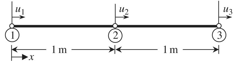
Consider a finite element with three nodes, as shown in the figure. When the solution is approximated using
Want to see the full answer?
Check out a sample textbook solution
Chapter 2 Solutions
Introduction To Finite Element Analysis And Design


- Solve the initial value problem. y" + 4y' + 20y = 0: y(0) = 2 y (0) = - 3 %3D Chapter 6, Section 6.2, Go Tutorial Problem 12 Find Y(s). 2s + 5 Y(s): s2 + 4s + 20 2s + 5 Y(s) = s2 + 4s + 20 2s – 5 Y(s) : + 4s + 20 2 + 4s + 20 Y(s) 2s + 5arrow_forward2. Solve the system linear of Equation using Gauss- Jordan elimination (row operations), find the value of x1, x2 and x3. 2X1 - 2X2 + X3 = 3 3X1 - X3 + X2 = 7 X1 - 3X2 + 2X3 = 0arrow_forward(3) For the given boundary value problem, the exact solution is given as = 3x - 7y. (a) Based on the exact solution, find the values on all sides, (b) discretize the domain into 16 elements and 15 evenly spaced nodes. Run poisson.m and check if the finite element approximation and exact solution matches, (c) plot the D values from step (b) using topo.m. y Side 3 Side 1 8.0 (4) The temperature distribution in a flat slab needs to be studied under the conditions shown i the table. The ? in table indicates insulated boundary and Q is the distributed heat source. I all cases assume the upper and lower boundaries are insulated. Assume that the units of length energy, and temperature for the values shown are consistent with a unit value for the coefficier of thermal conductivity. Boundary Temperatures 6 Case A C D. D. 00 LEGION Side 4 z episarrow_forward
- Q1: Find the Laplace inverse for the function 8 3 F(s) = 3 s2 + 12 s2 – 49 Q2: Solve IVP y" – 10y' + 9y = 5t ,y(0) = -1 and y'(0) = 2 %3D %3Darrow_forward3. Using the trial function u¹(x) = a sin(x) and weighting function w¹(x) = b sin(x) find an approximate solution to the following boundary value problems by determining the value of coefficient a. For each one, also find the exact solution using Matlab and plot the exact and approximate solutions. (One point each for: (i) finding a, (ii) finding the exact solution, and (iii) plotting the solution) a. (U₁xx -2 = 0 u(0) = 0 u(1) = 0 b. Modify the trial function and find an approximation for the following boundary value problem. (Hint: you will need to add an extra term to the function to make it satisfy the boundary conditions.) (U₁xx-2 = 0 u(0) = 1 u(1) = 0arrow_forwardFrom the following graph identify the steady-state maximum force. 1.2 1 0.8 0.6 0.4 0.2 0 Electical Power 1 Force vs. Time 2 Time (s) m 4 5arrow_forward
- please solve it in clear note: The fifth section solved it by using MATLAB i need all qusestion solved 1-9 For the mass spring damper system shown in the figure, assume that m = 0.25 kg, k= 2500 N/m, and c = 10 N.s/m. The values of force measured at 0.05-second intervals in one cycle are given below. 0.05 0.10 0.15 0.20 0.25 0.30 0.35 0.40 time F(t) time 12 14 44 19 33 34 12 22 0.60 25 0.45 0.50 0.55 0.65 0.70 0.75 0.80 0.85 Force 32 11 18 30 49 40 35 21 time 0.90 0.95 F(t) 11 m +x F(1) 1- Find the equation of motion. 2- Find the homogenous solution. 3- If we excite the system with initial displacement and velocity as 5 mm and 0.2 m/s respectively, plot the response of the free vibration system. 4- Use the generated plot in part 3 to verify the value of the damping constant, c. 5- Find the steady state solution (only particular solution) for the forced vibration system. Take number of terms in your Fourier series terms from this range [ 30 – 55). 6- Plot the force in the table, and the…arrow_forwardQ3) Find the optimal solution by using graphical method:. Max Z = x1 + 2x2 Subject to : 2x1 + x2 < 100 X1 +x2 < 80 X1 < 40 X1, X2 2 0arrow_forward3. Using the trial function uh(x) = a sin(x) and weighting function wh(x) = b sin(x) find an approximate solution to the following boundary value problems by determining the value of coefficient a. For each one, also find the exact solution using Matlab and plot the exact and approximate solutions. (One point each for: (i) finding a, (ii) finding the exact solution, and (iii) plotting the solution) a. (U₁xx - 2 = 0 u(0) = 0 u(1) = 0 b. Modify the trial function and find an approximation for the following boundary value problem. (Hint: you will need to add an extra term to the function to make it satisfy the boundary conditions.) (U₁xx - 2 = 0 u(0) = 1 u(1) = 0arrow_forward
 Elements Of ElectromagneticsMechanical EngineeringISBN:9780190698614Author:Sadiku, Matthew N. O.Publisher:Oxford University Press
 Mechanics of Materials (10th Edition)Mechanical EngineeringISBN:9780134319650Author:Russell C. HibbelerPublisher:PEARSON
 Thermodynamics: An Engineering ApproachMechanical EngineeringISBN:9781259822674Author:Yunus A. Cengel Dr., Michael A. BolesPublisher:McGraw-Hill Education
 Control Systems EngineeringMechanical EngineeringISBN:9781118170519Author:Norman S. NisePublisher:WILEY
 Mechanics of Materials (MindTap Course List)Mechanical EngineeringISBN:9781337093347Author:Barry J. Goodno, James M. GerePublisher:Cengage Learning
 Engineering Mechanics: StaticsMechanical EngineeringISBN:9781118807330Author:James L. Meriam, L. G. Kraige, J. N. BoltonPublisher:WILEY