
Concept explainers
Videos
Pillar stability is a most important factor to ensure safe conditions in underground mines. The authors of “Developing Coal Pillar Stability Chart Using Logistic Regression” (Intl. J. of Rock Mechanics & Mining Sci., 2013: 55–60) used a logistic regression model to predict stability. The article reported the following data on x1 = pillar height to width ratio, x2 = pillar strength to stress ratio, and stability status for 29 coal pillars.
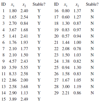
The corresponding logistic regression output from R is given here:
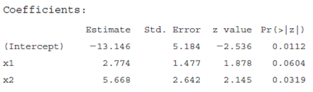
a. Using the output with α = .1 to determine whether the two predictor variables appear to have a significant impact on pillar stability.
b. Provide interpretations for e2.774 and e5.668.

Trending nowThis is a popular solution!

Chapter 13 Solutions
Probability and Statistics for Engineering and the Sciences


- Explain which characteristic of the STA leads to a consideration of a logistic model as opposed to a linear regression mode.arrow_forwardPlease use SPSS to solve! This exercise requires the use of a computer pack-age. The article “Movement and Habitat Use by Lake Whitefish During Spawning in a Boreal Lake: Inte-grating Acoustic Telemetry and Geographic Informa-tion Systems” (Transactions of the American Fisheries Society [1999]: 939–952) included the accompanying data on 17 fish caught in 2 consecutive years. a. Fit a multiple regression model to describe the rela-tionship between weight and the predictors length and age. y^5 2 511 1 3.06 length 2 1.11 ageb. Carry out the model utility test to determine whether at least one of the predictors length and age are useful for predicting weight.arrow_forwardThis dataset continues our saga of modeling the price of this popular Honda automobile. The dataset has now been cleaned to remove the columns with the dealership where the car was offered for sale and specific trim. (a) write out your model in econometric notation. Be very precise! (b) using the 93 observations in the dataset, estimate a model where price is a function of age, mileage and trim of the car. Be sure to avoid the dummy variable trap!! Fully report the results of your model. In this case, interpretation of the coefficients on the dummy variables is particularly important. (c) test the hypothesis that the specific trim does not affect the price of a Civic. Be sure to do all parts of the hypothesis test. (please fully describe steps if you are using Excel) Price Years Old KM EX EXT SE Sport Touring 6555 9 290363 0 0 0 0 0 9999 9 142258 0 0 0 0 0 10281 6 132644 0 0 0 0 0 12480 5 167125 0 0 0 0 0 12991 7 57398 0 0 0 0 0 12991 6 93046 0 0 0 0 0 12991…arrow_forward
- a) We conduct a regression of size on hhinc, owner, hhsize, hhsize2,and hhsize3. We do not include the constant. The regression output is reported in Table 3. Would you conclude that the home size increases with the household size? Interpret the sign and magnitude of the estimated coefficients of hhsize1, hhsize2, and hhsize3.arrow_forwardThe ages (X) of ten second-hand cars and their km values (Y) are given below.a) Calculate the correlation coefficient between X and Y.b) Calculate the coefficients of the regression line of the Y with respect to X.c) Estimate the km value of a 5.0 year old car. X and Y values given in the picture.arrow_forwardThe article "Earthmoving Productivity Estimation Using Linear Regression Techniques" (S. Smith, Journal of Construction Engineering and Management, 1999:133–141) presents the following linear model to predict earth-moving productivity (in m3 moved per hour): Productivity = - 297.877 + 84.787x, + 36.806x, + 151.680x, – 0.081x, – 110.517x5 - 0.267.x, – 0.016x,x, +0.107.x,x5 + 0.0009448x,x, – 0.244x;x, where X1 = number of trucks X2 = number of buckets per load X3 = bucket volume, in m³ X4 = haul length, in m X5 = match factor (ratio of hauling capacity to loading capacity) X6 = truck travel time, in s If the bucket volume increases by 1 m², while other independent variables are unchanged, can you determine the change in the predicted productivity? If so, determine it. If not, state what other information you would need to determine it. b. If the haul length increases by 1 m, can you determine the change in the predicted productivity? If so, determine it. If not, state what other…arrow_forward
- Which of the non-parametric test for ordinal data is the best to use in the given scenario? An experiment was conducted to compare the strengths of two types of elastic bandages: one a standard bandage of a specified weight and the other the same standard but treated with a chemical substance. Ten pieces of each were randomly selected from production. Does the treated bandage tend to be stronger than the standard? Table 1. Strength measurements (and their ranks) for 2 types of bandages. STANDARD TREATED 1.21(2) 1.49(15) 1.43(12) 1.37(7.5) 1.35(6) 1.67(20) 1.51(17) 1.50(16) 1.39(9) 1.31(5) 1.17(1) 1.29(3.5) 1.48(14) 1.52(18) 1.42(11) 1.37(7.5) 1.29(3.5) 1.44(13) 1.4(10) 1.53(19) a. Mood median test b. sign test c. Wilcoxon rank-sum test d. Wilcoxon matched-pairs signed-ranks test e. Spearman and Kendall correlation coefficients f. Kruskal-Wallis testarrow_forwardAssume we have data demonstrating a strong linear link between the amount of fertilizer applied to certain plants and their yield. Which is the independent variable in this research question?arrow_forwardThe depth of wetting of a soil is the depth to which water content will increase owing to extemal factors. The article "Discussion of Method for Evaluation of Depth of Wetting in Residential Areas" (J. Nelson, K. Chao, and D. Overton, Journal of Geotechnical and Geoenvironmental Engineering, 2011:293-296) discusses the relationship between depth of wetting beneath a structure and the age of the structure. The article presents measurements of depth of wetting, in meters, and the ages, in years, of 21 houses, as shown in the following table. Age Depth 7.6 4 4.6 6.1 9.1 3 4.3 7.3 5.2 10.4 15.5 5.8 10.7 4 5.5 6.1 10.7 10.4 4.6 7.0 6.1 14 16.8 10 9.1 8.8 Compute the least-squares line for predicting depth of wetting (y) from age (x). b. Identify a point with an unusually large x-value. Compute the least-squares line that results from deletion of this point. Identify another point which can be classified as an outlier. Compute the least-squares line that results from deletion of the outlier,…arrow_forward
- The body mass index (BMI) of a person is defined to be the person’s body mass divided by the square of the person’s height. The article “Influences of Parameter Uncertainties within the ICRP 66 Respiratory Tract Model: Particle Deposition” (W. Bolch, E. Farfan, et al., Health Physics, 2001:378–394) states that body mass index (in kg/m²) in men aged 25–34 is lognormally distributed with parameters μ = 3.215 and σ = 0.157. a) Find the mean BMI for men aged 25–34. b) Find the standard deviation of BMI for men aged 25–34. c) Find the median BMI for men aged 25–34. d) What proportion of men aged 25–34 have a BMI less than 22? e) Find the 75th percentile of BMI for men aged 25–34.arrow_forwardAttached to the end of the page is a portion of a printout from a stepwise regression analysis. a) Any of the F statistics on the printout can be computed via the formula: F = (SSReg( Model A ) – SSReg( Model B ) ) / C MSResidual( Model A) Identify what Model A, Model B, and the constant C are in order to obtain the F = 1.33 value for the variable x8 . b) Based on the printout for Step 6 of the stepwise selection procedure, what will be the next change in the model, in Step 7 of the procedure? (In other words, will a particular term be dropped, or added, or will nothing occur? Assume that the significance level for entry and staying are a = .15.)arrow_forwardAa Febru The body mass index (BMI) of a person is defined to be the person's body mass divided by the square of the person's height. The article "Influences of Parameter Uncertainties within the ICRP 66 Respiratory Tract Model: Particle Deposition" (W. Bolch, E. Farfan, et al., Health Physics, 2001:378-394) states that body mass index (in kg/m2) in men aged 25-34 is lognormally distributed with parameters u = 3.215 and o = 0.157. a.Find the mean and standard deviation BMI for men aged 25-34. b.Find the standard deviation of BMI for men aged 25-34. c.Find the median BMI for men aged 25-34. d.What proportion of men aged 25-34 have a BMI less than 20? e.Find the 80th percentile of BMI for men agėd 25 -34. 04... Rext 田arrow_forward
 Calculus For The Life SciencesCalculusISBN:9780321964038Author:GREENWELL, Raymond N., RITCHEY, Nathan P., Lial, Margaret L.Publisher:Pearson Addison Wesley,