
Concept explainers
Videos
a.
Identify and explain whichof the given modelscan be recommended.
a.
Answer to Problem 66SE
The model with 2 predictors and the model with 3 predictors can be recommended for predicting the pH before addition of dyes.
Explanation of Solution
Given info:
The MINITAB output shows the best regression option for the data predicted for pH before the addition of dyes using carpet density, carpet weight, dye weight, dye weight as a percentage of carpet and pH after addition of dyes.
Justification:
Mallows
It is used to assess the fit of regression model where the aim to find the best subset of predictors. A relatively small value of
By observing the mallows
By examining the models with three variables,
Hence, the model with two predictorsnamely dye weight and pH after addition of dyes could be considered as a best model subset for predicting pH before the addition of dyes.
Also, a second option would be the model with three predictorsnamely carpet weight, dye weight and pH after addition of dyes could be considered as a best model subset for predicting pH before the addition of dyes.
b.
Test whether the model suggests a useful linear relationship between pH before the addition of dyes and at least one of the predictors.
b.
Answer to Problem 66SE
There is sufficient evidence to conclude that the there is a use of linear relationship between pH before the addition of dyes and at least one of the predictors dye weight and pH after the addition of dyes.
Explanation of Solution
Given info:
The MINITAB output for predicting the pH before the addition of dyes using the dye weight
Calculation:
The test hypotheses are given below:
Null hypothesis:
That is, there is no use of linear relationship between pH before the addition of dyes and the predictors dye weightand pH after the addition of dyes.
Alternative hypothesis:
That is, there is a use of linear relationship between pH before the addition of dyes and at least one of the predictors dye weightand pH after the addition of dyes.
Conclusion:
The P-value is 0.000 and the level of significance is 0.001.
The P-value is lesser than the level of significance.
That is
Thus, the null hypothesis is rejected.
Hence, there is sufficient evidence to conclude that there is a use of linear relationship between pH before the addition of dyes and at least one of the predictors dye weight and pH after the addition of dyes.
c.
Explain whether either one of the predictors could be eliminated from the model given that the other predictor is retained.
c.
Answer to Problem 66SE
No, either one of the predictors could not be eliminated from the model given that the other predictor is retained.
Explanation of Solution
Calculation:
For variable
Testing the hypothesis:
Null hypothesis:
That is, there is no use of linear relationship between pH before the addition of dyes and dye weightgiven that pH after addition of dyes was retained in the model.
Alternative hypothesis:
That is, there is a use of linear relationship between pH before the addition of dyes and dye weightgiven that pH after addition of dyes was retained in the model.
From the MINITAB output it can be observed that the P-value corresponding to the t statistic of
Conclusion:
The P-value is 0.000 and the level of significance is 0.001.
The P-value is lesser than the level of significance.
That is
Thus, the null hypothesis is rejected.
Hence, there is sufficient evidence to conclude that there is a use of linear relationship between pH before the addition of dyes and dye weight given that pH after addition of dyes was retained in the model.
For variable
Testing the hypothesis:
Null hypothesis:
That is, there is no use of linear relationship between pH before the addition of dyes and pH after addition of dyes given that dye weight was retained in the model.
Alternative hypothesis:
That is, there is a use of linear relationship between pH before the addition of dyes and pH after addition of dyes given that dye weight was retained in the model.
From the MINITAB output it can be observed that the P-value corresponding to the t statistic of
Conclusion:
The P-value is 0.000 and the level of significance is 0.001.
The P-value is lesser than the level of significance.
That is
Thus, the null hypothesis is rejected.
Hence, there is sufficient evidence to conclude that there is a use of linear relationship between pH before the addition of dyes and pH after addition of dyes given that dye weight was retained in the model.
Justification:
From the analysis it can be concluded that none of the variables can be eliminated from the model given that the other variable is already present in the model.
d.
Calculate and interpret the 95% confidence interval for the two predictors.
d.
Answer to Problem 66SE
The 95% confidence interval for the estimated slope coefficient
(–0.0000684, –0.0000244).
The 95% confidence interval for the estimated slope coefficient
Explanation of Solution
Calculation:
The 95% confidence interval is calculated using the formula:
The confidence interval is calculated using the formula:
Where,
n is the total number of observations.
k is the total number of predictors in the model.
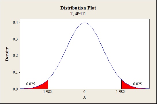
Critical value:
Software procedure:
Step-by-step procedure to find the critical value is given below:
- Click on Graph, select View Probability and click OK.
- Select t, enter 111 as Degrees of freedom, inShaded Area Tab select Probability under Define Shaded Area By and choose Both tails.
- Enter Probability value as 0.05.
- Click OK.
Output obtained from MINITAB is given below:
The 95% confidence interval for
Thus, the 95% confidence interval for the estimated slope coefficient
(–0.0000684, –0.0000244).
The 95% confidence interval for
Thus, the 95% confidence interval for the estimated slope coefficient
(0.6417,0.8325).
Interpretation:
For the variable
For one unit increase in the dye weight, it is 95% confident that the estimated value of pH before addition of dyes would decrease between–0.00000684 and–0.0000244 given that pH after addition of dyes is fixed constant.
For the variable
For one unit increase in the pH after the addition of dyes it is 95% confident that the estimated value of pH before addition of dyes would increase between 0.6417 and 0.8325 given that dye weight is fixed constant.
e.
Calculate and interpret the 95% confidence interval for the average value of pH before the addition of dyes when the dye weight and pH after the addition of dyes takes 1,000 and 6, respectively.
e.
Answer to Problem 66SE
The 95% confidence interval for the average value of pH before the addition of dyes when the dye weight and pH after the addition of dyes takes 1,000 and 6, respectively is (5.250, 5.383)
Explanation of Solution
Given info:
The estimated standard deviation for predicting the pH before the addition of dyes when the dye weight and pH after the addition of dyes takes 1,000 and 6 is 0.0336.
Calculation:
The average value of pH before the addition of dyes when the dye weight and pH after the addition of dyes takes 1,000 and 6 is calculated as follows:
Thus, the average value of pH before the addition of dyes when the dye weight and pH after the addition of dyes takes 1,000 and 6 is 5.316.
95% confidence interval for the true response:
The confidence interval is calculated using the formula:
Where,
n is the total number of observations.
k is the total number of predictors in the model.
Critical value:
Software procedure:
Step-by-step procedure to find the critical value is given below:
- Click on Graph, select View Probability and click OK.
- Select t, enter 111 as Degrees of freedom, in Shaded Area Tab select Probability under Define Shaded Area By and choose Both tails.
- Enter Probability value as 0.05.
- Click OK.
Output obtained from MINITAB is given below:
The 95% confidence interval is given below:
Thus, the 95% confidence interval for the average value of pH before the addition of dyes when the dye weight and pH after the addition of dyes takes 1,000 and 6 is (5.250,5.383).
Interpretation:
It is 95% confident that average value of pH before the addition of dyes when the dye weight and pH after the addition of dyes takes 1,000 and 6 would lie between 5.250 and 5.383.
Want to see more full solutions like this?
Chapter 13 Solutions
Probability and Statistics for Engineering and the Sciences


- Simple linear regression results: Dependent Variable: DIAMETER Independent Variable: RATO DIAMETER = -1314.0475 + 199.06132 RATO Sample size: 13 R (correlation coefficient) = 0.97602564 R-sq = 0.95262604 %3D Estimate of error standard deviation: 45.080042 Parameter estimates: Parameter Estimate Std. Err. Alternative DF T-Stat P-value Intercept -1314.0475 110.80982 11 -11.858583 <0.0001 Slope 199.06132 13.384407 11 14.872629 <0.0001 Analysis of variance table for regression model: Source DF SS MS F-stat P-value Model 1 449514.92 449514.92 221.19509 <0.0001 Error 11 22354.312 2032.2102 Total 12 471869.23arrow_forwardSnowpacks contain a wide spectrum of pollutants thatmay represent environmental hazards. The article“Atmospheric PAH Deposition: Deposition Velocitiesand Washout Ratios” (J. of EnvironmentalEngineering, 2002: 186–195) focused on the depositionof polyaromatic hydrocarbons. The authors proposeda multiple regression model for relating depositionover a specified time period (y, in mg/m2) to tworather complicated predictors x1 (mg-sec/m3) and x2 (mg/m2), defined in terms of PAH air concentrations forvarious species, total time, and total amount of precipitation.Here is data on the species fluoranthene andcorresponding Minitab output:obs x1 x2 flth1 92017 .0026900 278.782 51830 .0030000 124.533 17236 .0000196 22.654 15776 .0000360 28.685 33462 .0004960 32.666 243500 .0038900 604.707 67793 .0011200 27.698 23471 .0006400 14.189 13948 .0004850 20.6410 8824 .0003660 20.6011 7699 .0002290 16.6112 15791 .0014100 15.0813 10239 .0004100 18.0514 43835 .0000960 99.7115 49793 .0000896 58.9716 40656…arrow_forwardThe Cadet is a popular model of sport utility vehicle, known for its relatively high resale value. The bivariate data given below were taken from a sample of fifteen Cadets, each bought new two years ago, and each sold used within the past month. For each Cadet in the sample, we have listed both the mileage x (in thousands of miles) that the Cadet had on its odometer at the time it was sold used and the price y (in thousands of dollars) at which the Cadet was sold used. The least-squares regression line for these data has equation y = 40.63 - 0.46x . This line is shown in the scatter plot below. Mileage, x(in thousands) Used selling price, y(in thousands of dollars) 23.9 29.5 37.6 22.6 20.8 30.9 23.3 33.1 28.3 26.1 27.3 29.9 27.7 29.8 20.9 30.3 25.8 27.2 34.4 25.9 23.9 27.4 23.8 27.5 23.2 31.4 15.6 34.0 29.4 27.7 Send…arrow_forward
- A student collected concentration versus absorbance data for a series of standards and produced a standard curve. Which value of 2 would reflect the linear regression curve the student produced? Absorbance 1 0.9 0.8 0.7 0.6 0.5 0.4 0.3 0.2 0.1 0 0 ² = 0.10 ² = 0.76 ² = 0.98 2 = 0.45 1 Absorbance vs. Concentration 2 3 Concentration (ppm) 4 5 6arrow_forwardThe Cadet is a popular model of sport utility vehicle, known for its relatively high resale value. The bivariate data given below were taken from a sample of fifteen Cadets, each bought new two years ago, and each sold used within the past month. For each Cadet in the sample, we have listed both the mileage x (in thousands of miles) that the Cadet had on its odometer at the time it was sold used and the price y (in thousands of dollars) at which the Cadet was sold used. The least-squares regression line for these data has equation y=41.52-0.49x. This line is shown in the scatter plot below. Mileage, x (in thousands) 15.7 23.3 27.5 20.7 23.9 23.6 21.1 25.6 26.5 24.2 37.7 22.9 28.0 29.4 34.1 Send data to calculator V Used selling price, y (in thousands of dollars) Send data to Excel 34.5 33.9 29.9 31.2 26.9 27.3 31.4 26.4 30.8 30.3 22.8 30.5 25.9 28.1 25.5 Based on the sample data and the regression line, complete the following. Used selling price (in thousands of dollars) 40+ 35 30- 25-…arrow_forwardThe Cadet is a popular model of sport utility vehicle, known for its relatively high resale value. The bivariate data given below were taken from a sample of fifteen Cadets, each bought new two years ago, and each sold used within the past month. For each Cadet in the sample, we have listed both the mileage x (in thousands of miles) that the Cadet had on its odometer at the time it was sold used and the price y (in thousands of dollars) at which the Cadet was sold used. The least-squares regression line for these data has equation y = 40.86-0.45x. This line is shown in the scatter plot below. Mileage, x (in thousands) 29.7 27.8 26.8 24.2 21.1 23.0 24.3 15.4 37.7 23.6 34.4 27.8 23.5 20.9 259 Used selling price, y (in thousands of dollars) 27.4 29.4 31.2 30.1 31.7 31.7 27.2 34.2 23.4 28.2 26.3 26.5 33.7 30.6 267 Used selling price (in thousands of dollars) 40- 35+ 30- 25- 20 THIS 15 X 20 X X X 30 Mileagex (in thousands) X 35 40arrow_forward
- The Cadet is a popular model of sport utility vehicle, known for its relatively high resale value. The bivariate data given below were taken from a sample of sixteen Cadets, each bought new two years ago, and each sold used within the past month. For each Cadet in the sample, we have listed both the mileage x (in thousands of miles) that the Cadet had on its odometer at the time it was sold used and the price y (in thousands of dollars) at which the Cadet was sold used. The least-squares regression line for these data has equation Ŷ=42.80-0.53x. This line is shown in the scatter plot below. (The 2nd picture contains the rest of the data as it would not fit in the first pic and it includes the question as well.)arrow_forwardThe Cadet is a popular model of sport utility vehicle, known for its relatively high resale value. The bivariate data given below were taken from a sample of sixteen Cadets, each bought new two years ago, and each sold used within the past month. For each Cadet in the sample, we have listed both the mileage x (in thousands of miles) that the Cadet had on its odometer at the time it was sold used and the price y (in thousands of dollars) at which the Cadet was sold used. With the aim of predicting the used selling price from the number of miles driven, we might examine the least-squares regression line, Ŷ=42.39-0.52x. This line is shown in the scatter plot below. (The 2nd picture contains the rest of the data as it would not fit in the first pic and it includes the question as well.)arrow_forwardAn articie in Technometrics by S.C. Narula and J. F. Wallington Prediction, Lincar Regression, and a Minimum Sum of Relative Errors" Vol. 19, 1977) presents data on the sallingprica (y) and annual taas (x) for 24 houses. The taxes include local, school and county taxes. The data are shown in the following table. Sale Price/1000 Taxas/1000 25.9 4.9176 29.5 5.0208 27.9 4.5429 25.9 4.5573 29.9 5.0597 29.9 3.8910 30.9 5.8980 28.9 5.6039 35.9 5.8282 31.5 5.3003 31.0 6.2712 30.9 5.9592 30.0 5.0500 36.9 8.2464 41.9 6.6969 40.5 7.7841 43.9 9.0384 37.5 5.9894 37.9 7.5422 44.5 8.7951 37.9 6.0831 38.9 8.3607 36.9 8.1400 45.8 9.1416 (a) Calculate the least squares estimates of the slops and intercspt. (Round your answer to 3 decimal places.) (Round your answer to 2 decimal places.) (b) Find the mean selling price given that the taxes paid arex-8.9. (Round your answer to 2 decimal places.)arrow_forward
- The Cadet is a popular model of sport utility vehicle, known for its relatively high resale value. The bivariate data given below were taken from a sample of sixteen Cadets, each bought new two years ago, and each sold used within the past month. For each Cadet in the sample, we have listed both the mileage x (in thousands of miles) that the Cadet had on its odometer at the time it was sold used and the price y (in thousands of dollars) at which the Cadet was sold used. With the aim of predicting the used selling price from the number of miles driven, we might examine the least-squares regression line, y=42.91-0.54.x. This line is shown in the scatter plot below. Mileage, x (in thousands) 28.3 29.3 34.5 23.4 15.2 27.2 24.3 21.1 37.5 23.8 24.3 21.0 38.9 26.0 28.1 23.0 Used selling price, y (in thousands of dollars) 25.9 27.9 24.9 33.5 33.9 30.8 27.3 31.7 22.5 28.9 29.6 31.4 20.7 26.2 29.9 31.2 Send data to calc... ✔ Send data to Excel Used selling price (in thousands of dollars) 30+ 25-…arrow_forwardThe Cadet is a popular model of sport utility vehicle, known for its relatively high resale value. The bivariate data given below were taken from a sample of sixteen Cadets, each bought new two years ago, and each sold used within the past month. For each Cadet in the sample, we have listed both the mileage x (in thousands of miles) that the Cadet had on its odometer at the time it was sold used and the price y (in thousands of dollars) at which the Cadet was sold used. With the aim of predicting the used selling price from the number of miles driven, we might examine the least-squares regression line, y = 41.51-0.49x. This line is shown in the scatter plot below. Mileage, x (in thousands) Used selling price, y (in thousands of dollars) 24.2 27.6 26.9 30.0 28.1 25.5 40+ 20.5 30.4 15.5 34.5 21.1 31.0 24.1 29.8 30- 23.4 28.3 37.8 23.3 27.7 29.5 20- 23.6 33.2 39.3 21.3 23.3 31.3 Mileage (in thousands) 25.7 26.4 34.4 25.4 29.4 28.8 Send data to calculator Send data to Excel Based on the…arrow_forwardThe Cadet is a popular model of sport utility vehicle, known for its relatively high resale value. The bivariate data given below were taken from a sample of sixteen Cadets, each bought new two years ago, and each sold used within the past month. For each Cadet in the sample, we have listed both the mileage x (in thousands of miles) that the Cadet had on its odometer at the time it was sold used and the price y (in thousands of dollars) at which the Cadet was sold used. The least- squares regression line for these data has equation y=41.49 -0.48x. This line is shown in the scatter plot below. Mileage, x (in thousands) 21.1 28.1 34.3 15.5 27.3 22.6 24.4 27.8 39.2 37.9 25.8 23.7 24.5 23.4 29.7 20.7 Send data to calculator V Used selling price, y (in thousands of dollars) 32.0 26.5 26.0 33.5 30.5 29.9 30.5 30.4 21.5 22.8 26.5 27.8 27.7 34.1 27.8 31.0 Used selling price (in thousands of dollars) Based on the sample data and the regression line, complete the following. 40- 30- FINS (a) For…arrow_forward
 Calculus For The Life SciencesCalculusISBN:9780321964038Author:GREENWELL, Raymond N., RITCHEY, Nathan P., Lial, Margaret L.Publisher:Pearson Addison Wesley,
 Big Ideas Math A Bridge To Success Algebra 1: Stu...AlgebraISBN:9781680331141Author:HOUGHTON MIFFLIN HARCOURTPublisher:Houghton Mifflin Harcourt