Introductory Statistics (10th Edition)
10th Edition
ISBN: 9780321989178
Author: Neil A. Weiss
Publisher: PEARSON
expand_more
expand_more
format_list_bulleted
Concept explainers
Textbook Question
Chapter C.7, Problem 132E
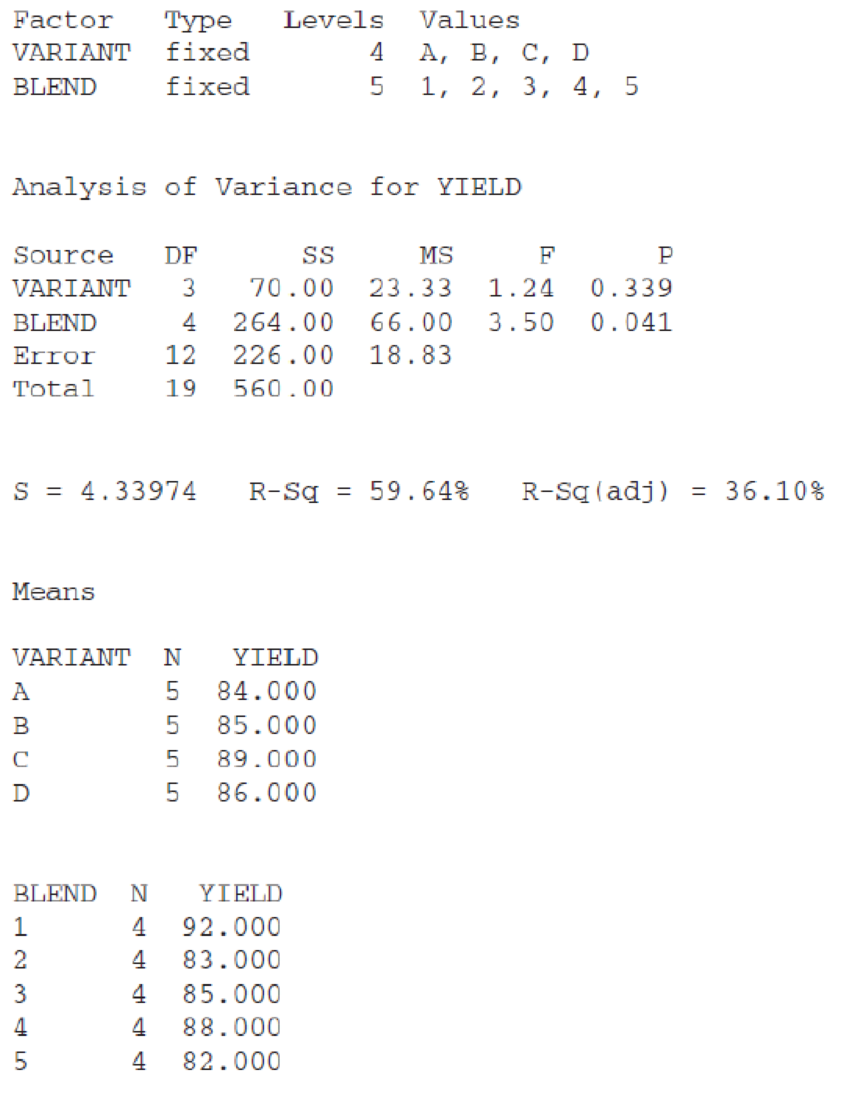
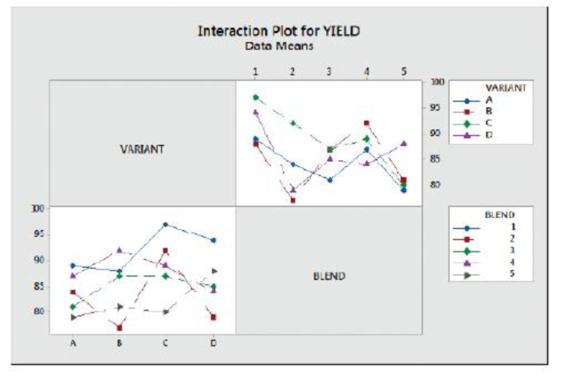
Penicillin Yields. Refer to Exercise C.121. Use the technology of your choice to obtain computer output similar to that in Outputs C.38 and C.39 on pages C-84 and C-85.
OUTPUT C.38
Output for Exercise C.121
(and Exercise C.128)
ANOVA: YIELD versus VARIANT, BLEND
OUTPUT C.39
Output for Exercise C.121
(and Exercise C.128)
Expert Solution & Answer
Want to see the full answer?
Check out a sample textbook solution
Students have asked these similar questions
5h.
David's Landscaping has collected data on home values (in thousands of $) and expenditures (in thousands of $) on landscaping with the hope of developing a predictive model to help marketing to potential new clients. Data for 14 households may be found in the file Landscape.
HomeValue($1,000)
LandscapingExpenditures($1,000)
242
8.1
321
10.8
198
12.2
340
16.2
300
15.6
400
18.9
800
23.5
200
9.5
521
17.5
547
22.0
437
12.1
464
13.5
635
17.9
356
13.9
(c)
Use the least squares method to develop the estimated regression equation. (Let x = home value (in thousands of $), and let y = landscaping expenditures (in thousands of $). Round your numerical values to five decimal places.)
ŷ =
(d)
For every additional $1,000 in home value, estimate how much additional will be spent (in $) on landscaping. (Round your answer to the nearest cent.)
$
(e)
Use the equation estimated in part (c) to predict the landscaping expenditures (in $) for a…
Use the advertised prices for used cars of a particular model in the accompanying table to create a linear model for the relationship between a car's Age and its Price.
Complete parts a through g.
E Click the icon to view the data table.
......
e) You have a chance to buy one of two cars. They are about the same age and appear to be in equally good condition. Would you rather buy the one with a positive
residual or the one with a negative residual? Explain.
O A. The car with a positive residual is better because its actual price is above the predicted price for its age.
Data table
O B. The car with a positive residual is better because its actual price is below the predicted price for its age.
OC. The car with a negative residual is better because its actual price is above the predicted price for its age.
Age (yr)
Price Advertised ($)
OD. The car with a negative residual is better because its actual price is below the predicted price for its age.
1
17,619
14,999
16,018
13,988
15,009…
7. Look at the graph "Black small businesses hit twice as hard as white ones". Estimate the percert of
white small businesses and self-employed workers who were not working in April 2020. Estimate the
percent of black small businesses and self-employed workers who were not working in April 2020. Is it
twice as much as the title claims?
99+
a
%23
近
Chapter C Solutions
Introductory Statistics (10th Edition)
Ch. C.1 - Define the following terms: a. factor b. levels of...Ch. C.1 - A three-way factorial design has Factor A at 3...Ch. C.1 - A four-way factorial design has Factor A at 2...Ch. C.1 - A three-way factorial design has Factor A at 6...Ch. C.1 - Answer true or false to each of the following...Ch. C.1 - Prob. 8ECh. C.1 - Answer true or false to each of the following...Ch. C.1 - Prob. 10ECh. C.1 - In each of Exercises C.11C.17 identify the...Ch. C.1 - In each of Exercises C.11C.17 identify the...
Ch. C.1 - In each of Exercises C.11C.17 identify the...Ch. C.1 - In each of Exercises C.11C.17 identify the...Ch. C.1 - In each of Exercises C.11C.17 identify the...Ch. C.1 - Prob. 16ECh. C.1 - In each of Exercises C.11C.17 identify the...Ch. C.2 - Consider a 3 4 ANOVA. a. Identify the number of...Ch. C.2 - Consider a 4 2 ANOVA. a. Identify the number of...Ch. C.2 - Prob. 25ECh. C.2 - Prob. 26ECh. C.2 - Prob. 27ECh. C.2 - Prob. 28ECh. C.2 - In two-way ANOVA, identify what we mean by a. a...Ch. C.2 - In two-way ANOVA, what does it mean we have...Ch. C.2 - In Exercises C.31C.33, we have presented partially...Ch. C.2 - Prob. 32ECh. C.2 - Prob. 33ECh. C.2 - Prob. 34ECh. C.2 - State the null and alternative hypotheses for a...Ch. C.2 - Prob. 36ECh. C.2 - In a two-way ANOVA, why is the test for...Ch. C.2 - Prob. 38ECh. C.2 - Prob. 39ECh. C.2 - Prob. 40ECh. C.2 - Prob. 41ECh. C.2 - Referring to Exercise C.38, for which part(s) is...Ch. C.2 - Prob. 43ECh. C.2 - Prob. 44ECh. C.2 - Prob. 45ECh. C.2 - Prob. 46ECh. C.3 - In each of Exercises C.47C.53, we have presented a...Ch. C.3 - In each of Exercises C.47C.53, we have presented a...Ch. C.3 - Prob. 49ECh. C.3 - Prob. 50ECh. C.3 - Prob. 51ECh. C.3 - Prob. 52ECh. C.3 - Prob. 53ECh. C.3 - Prob. 54ECh. C.3 - Prob. 55ECh. C.3 - Prob. 56ECh. C.3 - Prob. 57ECh. C.3 - Prob. 58ECh. C.3 - Prob. 59ECh. C.3 - Prob. 60ECh. C.3 - Prob. 61ECh. C.3 - Prob. 62ECh. C.3 - Prob. 63ECh. C.3 - Prob. 64ECh. C.3 - Prob. 65ECh. C.3 - Prob. 66ECh. C.3 - Prob. 67ECh. C.3 - Prob. 68ECh. C.3 - Prob. 69ECh. C.3 - Prob. 70ECh. C.3 - Prob. 71ECh. C.4 - In an experiment with two factors, A and B, what...Ch. C.4 - If the confidence interval for the difference...Ch. C.4 - Prob. 74ECh. C.4 - Prob. 75ECh. C.4 - Let Factor A have three levels and Factor B have...Ch. C.4 - In Exercises C.77C.83, we have repeated the...Ch. C.4 - Prob. 78ECh. C.4 - In Exercises C.77C.83, we have repeated the...Ch. C.4 - Prob. 80ECh. C.4 - In Exercises C. 77-C.83. we have repeated the...Ch. C.4 - In Exercises C.77C.83, we have repeated the...Ch. C.4 - Prob. 83ECh. C.4 - Household Income. Refer to Exercise C.77. Use the...Ch. C.4 - Prob. 85ECh. C.4 - Prob. 86ECh. C.4 - Highway Signs. Refer to Exercise C.80. Use the...Ch. C.4 - Hospital Stays. Refer to Exercise C.81. Use the...Ch. C.4 - Prob. 89ECh. C.4 - Advertising and Sales. Refer to Exercise C.83. Use...Ch. C.5 - In each of Exercises C.91C.97, identify the...Ch. C.5 - Prob. 92ECh. C.5 - In each of Exercises C.91C.97, identify the...Ch. C.5 - In each of Exercises C.91C.97, identify the...Ch. C.5 - In each of Exercises C.91C.97, identify the...Ch. C.5 - In each of Exercises C.91C.97, identify the...Ch. C.5 - In each of Exercises C.91C.97, identify the...Ch. C.6 - What is the purpose of blocking in a randomized...Ch. C.6 - Prob. 104ECh. C.6 - Prob. 105ECh. C.6 - Prob. 106ECh. C.6 - Answer true or false to the following statements...Ch. C.6 - Prob. 108ECh. C.6 - In randomized block ANOVA, what is meant when we...Ch. C.6 - Prob. 110ECh. C.6 - State the null and alternative hypotheses for a...Ch. C.6 - Identify, give the degrees of freedom for, and...Ch. C.6 - Prob. 113ECh. C.6 - Prob. 114ECh. C.6 - Prob. 115ECh. C.6 - Prob. 116ECh. C.6 - Prob. 117ECh. C.6 - Prob. 118ECh. C.7 - In each of Exercises C.119C.125, we have presented...Ch. C.7 - Prob. 120ECh. C.7 - Prob. 121ECh. C.7 - Prob. 122ECh. C.7 - Prob. 123ECh. C.7 - Prob. 124ECh. C.7 - Prob. 125ECh. C.7 - Prob. 126ECh. C.7 - Prob. 127ECh. C.7 - Prob. 128ECh. C.7 - Prob. 129ECh. C.7 - Prob. 130ECh. C.7 - Prob. 131ECh. C.7 - Penicillin Yields. Refer to Exercise C.121. Use...Ch. C.7 - Prob. 133ECh. C.7 - Battery Lifetimes. Refer to Exercise C.123. Use...Ch. C.7 - Prob. 135ECh. C.7 - Prob. 136ECh. C.7 - Prob. 137ECh. C.7 - Prob. 138ECh. C.7 - Prob. 139ECh. C.7 - Prob. 140ECh. C.7 - Prob. 141ECh. C.7 - Golf Ball Driving Distances. Refer to Exercise...Ch. C.7 - Prob. 143ECh. C.7 - Analgesic Effectiveness. Refer to the analgesic...Ch. C.8 - In a randomized block experiment with treatment...Ch. C.8 - If the confidence interval for the difference...Ch. C.8 - The parameter v for the q-curve in a Tukey...Ch. C.8 - Prob. 148ECh. C.8 - Prob. 149ECh. C.8 - Prob. 150ECh. C.8 - Prob. 151ECh. C.8 - Prob. 152ECh. C.8 - Prob. 153ECh. C.8 - Prob. 154ECh. C.8 - Mileage for Gasoline Brands. Refer to Exercises...Ch. C.8 - Prob. 156ECh. C.8 - Prob. 157ECh. C.8 - Barley Variety Yields. Refer to Exercises C.125...Ch. C.8 - Prob. 159ECh. C.9 - Of which test is the Friedman test a nonparametric...Ch. C.9 - Prob. 161ECh. C.9 - Prob. 162ECh. C.9 - Prob. 163ECh. C.9 - Fill in the following blank: If the null...Ch. C.9 - Prob. 165ECh. C.9 - For a Friedman test to compare the means of six...Ch. C.9 - Prob. 167ECh. C.9 - In each of Exercises C.168C.I74, determine whether...Ch. C.9 - Prob. 169ECh. C.9 - Prob. 170ECh. C.9 - Prob. 171ECh. C.9 - Prob. 172ECh. C.9 - Prob. 173ECh. C.9 - Prob. 174ECh. C.9 - Prob. 175ECh. C.9 - Prob. 176ECh. C.9 - Prob. 177ECh. C.9 - Prob. 178ECh. C.9 - Prob. 179ECh. C.9 - Prob. 180ECh. C.9 - Prob. 181ECh. C - Discuss the differences between a designed...Ch. C - In a complete factorial design, how do you...Ch. C - Prob. 3RPCh. C - Prob. 4RPCh. C - Prob. 5RPCh. C - Prob. 6RPCh. C - Prob. 7RPCh. C - For a two-way ANOVA: a. List and interpret the...Ch. C - Prob. 9RPCh. C - Prob. 10RPCh. C - State the assumptions for a two-way ANOVA and...Ch. C - Prob. 12RPCh. C - Prob. 13RPCh. C - Prob. 14RPCh. C - This problem concerns multiple comparisons. a....Ch. C - Cereal Sales. Refer to Problem 13. Perform...Ch. C - Explain why it is sometimes preferable to employ a...Ch. C - For a randomized block ANOVA: a. List and...Ch. C - Prob. 19RPCh. C - Prob. 20RPCh. C - Prob. 21RPCh. C - Prob. 22RPCh. C - Prob. 23RPCh. C - Prob. 24RPCh. C - Prob. 25RPCh. C - Identify the nonparametric alternative to the...Ch. C - Explain the logic behind the Friedman test.Ch. C - Prob. 28RPCh. C - Prob. 29RPCh. C - Prob. 30RPCh. C - Prob. 31RPCh. C - Prob. 32RPCh. C - Prob. 33RPCh. C - Prob. 34RPCh. C - Prob. 35RPCh. C - Prob. 36RP
Knowledge Booster
Learn more about
Need a deep-dive on the concept behind this application? Look no further. Learn more about this topic, statistics and related others by exploring similar questions and additional content below.Similar questions
- Urban Travel Times Population of cities and driving times are related, as shown in the accompanying table, which shows the 1960 population N, in thousands, for several cities, together with the average time T, in minutes, sent by residents driving to work. City Population N Driving time T Los Angeles 6489 16.8 Pittsburgh 1804 12.6 Washington 1808 14.3 Hutchinson 38 6.1 Nashville 347 10.8 Tallahassee 48 7.3 An analysis of these data, along with data from 17 other cities in the United States and Canada, led to a power model of average driving time as a function of population. a Construct a power model of driving time in minutes as a function of population measured in thousands b Is average driving time in Pittsburgh more or less than would be expected from its population? c If you wish to move to a smaller city to reduce your average driving time to work by 25, how much smaller should the city be?arrow_forwardQ A business researcher is investigating the relationship between certain personality characteristics of s business owners and the businesses' growth potential over the next five years. The researcher randon selects 15 small business owners, administers the "Speed and Impatience" (X) and "Job Involvement subscales of the Jenkins Activity Survey, and then determines the "Growth Potential (Z) for the businesses. The resulting data are as follows. Speed and Impatience Job Involvement Growth Potential Y Z 4 3 5 7 4 6 9 10 8 9 8 10 7 7 8 3 3 7 4 4 3 2 2 3 5 7 4 4 4 1 1 2 6 Without using SPSS, compute the following descriptive items. 1) The mean of the variable Speed and Impatience 2) The median of the variable growth potential 3) The quartiles Q1, Q2, Q3 and the IQR of the variable Speed and Impatiencearrow_forwardA wood products firm uses leftover time at the end of each week to make goods for stock. Currently, there are two products on the list of items that are produced for stock: a chopping board and a knife holder. Both items require three operations: cutting, gluing, and finishing. The manager of the firm has collected the following data on these products: ------------------------------------------------------- Time per unit (minutes) Profit ---------------------------- Item per unit Cutting Gluing Finishing ------------------------------------------------------- Chopping board $ 4 1.4 5 12 Knife holder $ 6 1.8 13 3 ------------------------------------------------------- The manager has also determined that during each week 120 minutes are available for cutting, 650 minutes are available for gluing, and 360…arrow_forward
- E BUSS 106 Excel Modified Spring 2019-2ON.pdf (page 31 of 43)- Edited Business Applications using Excel- Activity 9- Test your learning Instructions to the student: 1. Open a new excel file 2. Create a table for the following data in Excel. 3. Save the file as "BUSS 106 Excel Activity 12" Total Grades Both Sexes Female Male Kindergarten 75,384 3183 38,201 Basic education First episode 210.269 103,636 06.633 Basic education Second episode 128,193 15.338 General Education 343 317 Grades (1) Gemeral Edtucation Grades (5 10 1615. S.169 S.006 After Basic Education Grades (11-125 S(232 41.142 43,090 Grades (1-6) 31.031 15.018 16,013 Grades (79) 11.796 5,629 6167 Grades (19 12 7.803 3.473 4330 Total 701,0s1 342986 358,095 1. Calculate the percentage of males and females in each category. 2. Calculate the distribution percentage of students in each category gender wise. 3. Make a bar chart for the distribution percentage of males in each category. 31 282 APRarrow_forward10a,10b,&10carrow_forwardRefer to the ANOVA output below. A business researcher is investigating the process inputs that influence late orders (measured as % late). Which statement is FALSE? 1. Three factors are being researched simultaneously 2. There is a chance of a beta error in this analysis 3. Four different product types were considered in this research 4. Particular combinations (interactions) of Order Frequency and Quantity significantly influences late orders 5. The Order Frequency significantly influences whether an order is latearrow_forward
- 11 of 17 > Identify the ethical issue posed by each clinical trial. In 1932, an experiment was initiated at Tuskegee institute to study the effects of syphilis in African- American men if left untreated. The men were not told of the real purpose of the clinical trial and those afflicted with syphilis were not told of their diagnosis. Rather, they were led to believe that they were being treated for "bad blood", a colloquial term used to describe an assortment of ailments. The men were incentivized to participate in the trial with offers of free doctor visits and treatments. The experiment continued for 40 years and when syphilis treatment became available during the study timeframe, the treatment was witheld. In 1999, Jessie Gelsinger, a patient in a gene trial being conducted at the University of Pennsylvania, passed away shortly after taking the experimental therapy developed for a rare, genetic metabolic disorder. The researchers had previously told Jessie and his family that the…arrow_forwardReWritable DVD DVD+ReWritable MULTI RECORDER Esc F1 F2 F3 F4 F5 F6 Tab 3. A simple random sample of beachfront condo listings in Myrtle Beach comparing weekly rent ($) and size (square feet) yileds the following computer output. Lock 150 1800 75- 1500 1200 -75 900- 900 1200 15o0 2000 .. 600 1000 1250 1500 1750 2000 Size Predicted Rent to Coef -311.341 07ר1.07 s.e. Coef 117.6 0.09047 -2.65 11.9 = 94.0% 0.0294 0.0001 Variable Conatant Size = 94.78 R-squ (adj) 102.4 R-aqu %3D Is a linear model appropriate for these data? Explain. b) What is the equation for the least squares regression line? Define the varaibles within your equation. c) Interpret the slope of the regression line. c) Interpret r² in context. Ultra S SS CLL %24 2.arrow_forwardYou may need to use the appropriate technology to answer this question. An automobile dealer conducted a test to determine if the time in minutes needed to complete a minor engine tune-up depends on whether a computerized engine analyzer or an electronic analyzer is used. Because tune-up time varies among compact, intermediate, and full-sized cars, the three types of cars were us blocks in the experiment. The data obtained follow. Analyzer Computerized Electronic Compact 50 41 Car Intermediate 54 44 Full-sized 64 47 Use a = 0.05 to test for any significant differences. State the null and alternative hypotheses. O Ho: MCompact = "Intermediate = "Full-sized H: "Compact *"Intermediate * Full-sized O Ho: "Compact * "Intermediate * Full-sized H: "Compact = "Intermediate "Full-sized O Ho: "Computerized = HElectronic H: "Computerized * "Electronic O Ho: "Computerized = "Electronic = "Compact = 4Intermediate = "Full-sized H: Not all the population means are equal. O Ho: "Computerized *…arrow_forward
- A state's park system statistical report for the 2014/2015 fiscal year gave the accompanying data on x = amount of money collected in user fees (in thousands of dollars) and y = operating cost (in thousands of dollars) for nine state parks in a certain district. y 4000 3000 2000 1000 User Fees (thousands of dollars) y 4000 3000 2000 1000 17 74 (a) Construct a scatterplot of these data. 811 380 33 427 500 734 760 200 200 400 Operating Costs (thousands of dollars) 400 + 600 600 101 355 3,546 1,391 243 752 1,054 2,227 1,604 800 800 Describe any interesting features of the scatterplot. There is a positive X y 4000 3000 2000 1000 0 y 4000 3000 2000 1000 200 200 400 400 (b) Find the equation of the least squares line. (Round your answers to four decimal places.) ŷ = 600 600 linear relationship between user fees collected and operating costs. 800 800arrow_forwardTwo of the hottest smartphones on the market are the newly released iPhone6 and the Samsung Galaxy S6. CNet.com offers online reviews of all major cell phones, including battery life tests. In a review of the iPhone6, the talk-time battery life of 35 iPhones was measured. Similarly, the talk-time battery life of 30 Galaxy S6s was measured. Two outputs are given below. Which is appropriate for analyzing the data collected? Output 1 Output 2 Using the StatCrunch output chosen above, determine if there is a difference in the mean battery life for the two phones. Use a significance level of 0.01 when conducting the test. Select the appropriate hypotheses. Make sure the notation used in the hypotheses agrees with the type of samples selected in the output. Ho:μd=0Ho:μd=0Ha:μd<0Ha:μd<0 Ho:μd=0Ho:μd=0Ha:μd≠0Ha:μd≠0 Ho:μd=0Ho:μd=0Ha:μd>0Ha:μd>0 Ho:μ1=μ2Ho:μ1=μ2Ha:μ1>μ2Ha:μ1>μ2 Ho:μ1=μ2Ho:μ1=μ2Ha:μ1≠μ2Ha:μ1≠μ2 Ho:μ1=μ2Ho:μ1=μ2Ha:μ1<μ2Ha:μ1<μ2 αα =…arrow_forwardHow would you interpret the given output? Variables Cronbach’s Alpha Discriminant validity Brand Image Brand Loyalty Brand Awareness Brand Equity Brand Image 0.891 0.879 Brand Loyalty 0.809 0.405 0.949 Brand Awareness 0.836 0.21 0.183 0.878 Brand Equity 0.952 0.145 0.36 0.198 0.872arrow_forward
arrow_back_ios
SEE MORE QUESTIONS
arrow_forward_ios
Recommended textbooks for you
 Big Ideas Math A Bridge To Success Algebra 1: Stu...AlgebraISBN:9781680331141Author:HOUGHTON MIFFLIN HARCOURTPublisher:Houghton Mifflin Harcourt
 Linear Algebra: A Modern IntroductionAlgebraISBN:9781285463247Author:David PoolePublisher:Cengage Learning
 Glencoe Algebra 1, Student Edition, 9780079039897...AlgebraISBN:9780079039897Author:CarterPublisher:McGraw Hill
 Functions and Change: A Modeling Approach to Coll...AlgebraISBN:9781337111348Author:Bruce Crauder, Benny Evans, Alan NoellPublisher:Cengage Learning

Big Ideas Math A Bridge To Success Algebra 1: Stu...
Algebra
ISBN:9781680331141
Author:HOUGHTON MIFFLIN HARCOURT
Publisher:Houghton Mifflin Harcourt

Linear Algebra: A Modern Introduction
Algebra
ISBN:9781285463247
Author:David Poole
Publisher:Cengage Learning

Glencoe Algebra 1, Student Edition, 9780079039897...
Algebra
ISBN:9780079039897
Author:Carter
Publisher:McGraw Hill

Functions and Change: A Modeling Approach to Coll...
Algebra
ISBN:9781337111348
Author:Bruce Crauder, Benny Evans, Alan Noell
Publisher:Cengage Learning
Probability & Statistics (28 of 62) Basic Definitions and Symbols Summarized; Author: Michel van Biezen;https://www.youtube.com/watch?v=21V9WBJLAL8;License: Standard YouTube License, CC-BY
Introduction to Probability, Basic Overview - Sample Space, & Tree Diagrams; Author: The Organic Chemistry Tutor;https://www.youtube.com/watch?v=SkidyDQuupA;License: Standard YouTube License, CC-BY