
Concept explainers
Videos
Figure P8.44 shows three reservoirs connected by circular pipes. The pipes, which are made of asphalt-dipped cast iron
| Pipe | 1 | 2 | 3 |
| Length, m | 1800 | 500 | 1400 |
| Diameter, m | 0.4 | 0.25 | 0.2 |
| Flow,
|
|
0.1 | ? |
If the water surface elevations in Reservoirs A and C are 200 and 172.5 m, respectively, determine the elevation in Reservoir B and the flows in pipes 1 and 3. Note that the kinematic viscosity of water is
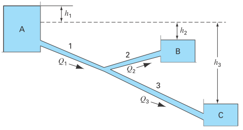
FIGURE P8.44
To calculate: The elevation in reservoir B and the flow in pipe 1 and pipe 3 in Figure P8.44, if the surface of water elevations in Reservoirs A is
Answer to Problem 44P
Solution:
The elevation in reservoir B is
The flow in pipe 1 is
The flow in pipe 3 is
Explanation of Solution
Given Information:
The pipe material is asphalt-dipped cast iron whose
The characteristics of the pipeare,
| Pipe | 1 | 2 | 3 |
| Length, m | 1800 | 500 | 1400 |
| Diameter, m | 0.4 | 0.25 | 0.2 |
| Flow, |
? | 0.1 | ? |
The surface of water elevations in Reservoirs A is
The kinematic viscosity of water is
To determine the friction factor, use the Colebrook equation (recall the Prob. 8.13).
Formula Used:
Write the Colebrook Equation to calculate the friction factor
Here,
Write the Blasius formula to find an initial approximation of the friction factor,
Write the Newton Raphson formula.
Write the expression for pressure drop in the section Pipe
Here,
Write the expression for the pressure.
Here,
Calculation:
Recall the characteristics of pipe,
| Pipe | 1 | 2 | 3 |
| Length, m | 1800 | 500 | 1400 |
| Diameter, m | 0.4 | 0.25 | 0.2 |
| Flow, |
? | 0.1 | ? |
Recall the Colebrook Equation.
Rearrange the Colebrook Equation for root location.
Here, Roughness is
Diameter is
Re is the Reynolds number
At initial approximation for Re is taken to be
Substitute all the above value in Colebrook Equation.
Calculate an initial approximation of the friction factor.
Recall the Blasius formula.
The initial estimation of Reynolds number is
Use the Newton Raphson method to find the root of the equation (2).
The function is as follows,
Take the first derivative.
Recall the Newton Raphson formula.
The iterations are shown below:
The root of the Equation occurs at
Calculate the pressure drop in the section Pipe 1.
Recall the expression for pressure drop in the section Pipe.
And the expression for the velocity of the circular pipe is,
Substitute
Now for pipe 1,
The frictional factor is
The length of the pipe is
Density is
Diameter is
Substitute all the value.
Rearrange for
Calculate the water pressure.
Write the expression for the water pressure.
The density of water is
And, this is equal to
Substitute
Therefore, the flow rate of pipe 1 is
Calculate the flow rate for the Pipe 3.
Substitution the roughness is
Calculate an initial approximation of the friction factor.
Recall the Blasius formula.
The initial estimation of Reynolds number is
Use the Newton Raphson method to find the root of the equation (4).
Write the function as follows,
Take the first derivative,
The iterations are shown below:
The root of the Equation occurs at
Calculate the pressure drop in the section Pipe 3.
Recall the expression for pressure drop in the section Pipe.
And the expression for the velocity of the circular pipe is,
Substitute
Now for pipe 3,
The frictional factor is
The length of the pipe is
Density is
Diameter is
Substitute all the value.
Rearrange for
The formula for water pressure is:
The density of water is
And, this is equal to
Substitute
Therefore, the flow rate of pipe 3 is
For Pipe 2,
Write the Colebrook Equation for root location from equation (1).
The roughness is
Substitution of the above parameters gives the following equation,
Calculate an initial approximation of the friction factor.
Recall the Blasius formula.
The initial estimation of Reynolds number is
The Newton Raphson formula is,
Use the Newton Raphson method to find the root of the equation (7).
Write the function as follows,
Take the first derivative,
The iterations are shown below:
The root of the Equation occurs at
Calculate the pressure drop in the section Pipe 2.
Recall the expression for pressure drop in the section Pipe.
And the expression for the velocity of the circular pipe is,
Substitute
Now for pipe 2,
The frictional factor is
The length of the pipe is
Density is
Diameter is
Substitute all the above value.
Now, this pressure drop in a section of Pipe 2 is equivalent to the water pressure from reservoir 2.
The formula for water pressure is,
Here, the density of water is
And, this is equal to
Substitute
Therefore, the elevation in reservoir B is
Want to see more full solutions like this?
Chapter 8 Solutions
EBK NUMERICAL METHODS FOR ENGINEERS
Additional Engineering Textbook Solutions
Fundamentals of Differential Equations (9th Edition)
Advanced Engineering Mathematics
Basic Technical Mathematics
High School Math 2012 Common-core Algebra 1 Practice And Problem Solvingworkbook Grade 8/9
Introductory Statistics (2nd Edition)


- Three pipes A, B, and C are interconnected as shown in figure 1. The pipe dimensions are as follows: D (cm) 15 10 20 Pipeline A L (m) 300 240 600 0.01 0.01 0.005 A 15 m 25 m В C Figure 1 1.1 Find the rate at which water will flow in each pipe, ignoring the shock losses at P and entry to pipelines A and B. 1.2 Find the pressure at P.arrow_forwardWater flows from a 20-mm-diameter pipe with a flowrate Q as shown in the figure below. What is the approximate diameter of the water stream, d, in units of cm, if the distance below the faucet is, h=2 m, and Q = 0.003 m³ /s? 20 mm O a. 1.83 m b. 2.07 m O c. 3.29 m d. 4.66 m O e. 5.29 marrow_forwardAn aqueduct is required to supply water to the community.Data: Families = 12 Average members per family = 3 people Breakfast, lunch and dinner = 15 total liters / family Showers = 10lt / person, one daily shower Kitchen wash = 13lts / day Total distance of the pipeline to the storage tank = 1200 meters Total height H from the pump point to delivery to the tank = 70 meters Determine: Estimation of the total volume of the recommended tank, an autonomy of at leas 2 days of storage. It is required to propose a pump that allows at least filling the tank between 5 to 12 hours operation, it must include details of the pump, as well as its curve Image: schematic detail of the proposed systemarrow_forward
- You were asked to design a water storage tank for your processing plant. The tank is cylindrical-shaped tank with diameter of 8.0 m. The water is to be supplied by a horizontal pipe (internal radius, ri = 6.00 cm), where water is under initial pressure of 2.00 atm., and flowrate of 2.0 m²/s. A vertical pipe (internal radius, rɔ = 1.00 cm) is to carry the water to a height of 9.40 m, where it is to pour out freely into the tank until the depth is 2.00 m. Assume water density of 1000 kg/m³, and g = 9.81m²/s. i) Calculate the volumetric flowrate and pressure at the pipe outflow.arrow_forward2. A storage contains liquid at depth y where y-0 when the tank is half full, as shown below. Liquid is withdrawn at a constant flow rate Q to meet demands. The contents are resupplied at a sinusoidal rate 3Qsin2(t). The storage tank has a diameter D=5m. a. Beginning from conservation of mass, formulate an equation for the change in dV TD2 depth of water as a function of time. Hint: dt din - 9out and V = 4 b. Use Euler's method to solve for the depth y, show the iterative equation for the Euler's method, and use Q=5 m3/s to complete the table below: t (s) y (m) 0.5 1.0arrow_forwardQ1. Two pumps with 105.4 cm in diameters characteristics shown in figure below are used in paralel to pump water to the system. Neglecting local losses, calculate total flow rate and pump power. (a) n= 710 d/dak 120 7.5 80m ENPY (2) 6. 105 - 105.4 cm çap S N 4.5 3 90 96.52 cm çap 88% 86% 75 - 88.9 cm çap S4% (1) bom 60 1100 kW 45 750 kW 30 0.25 0.50 0.75 1.00 1.25 1.50 1.75 Debi m/s Note: Pipe is cast iron with 0.6 m in diamater and 1.6 km in length. Fluid is water with density 1000 kg/m³ . ENPY m %68 900 kWarrow_forward
- A pumping station wet well operates between 540- and 550-ft elevation. The pump curve is deϐined by the following points: 80 ft at zero ϐlow, 78 ft at 200 gpm, 65 ft at 800 gpm, and 50 ft at 1200 gpm. The pump discharge contains an equivalent of 50 ft of 6-in. pipe. The discharge pipe is 120-ft long and terminates at a splitter box, elevation 570. Using C=100, plot the pump curve and the corrected pump curve. Plot the pump discharge curves at each wet well elevation and for C=100 and C=140. What is the pump ϐlow at the low and high wet well elevations for newand old pipe?arrow_forward1.28. The performance curve for the fan of Problem 1.27 can be approx- imated by a straight line through its BEP (using techniques devel- oped in Chapter 7). The curve is Aps = 4488 – 166Q, with ApT in Pa and Q in m³/s. If this fan is connected to a 1-m dia- meter duct (f = 0.045) whose length is 66 m, what flow rate will result? %3Darrow_forwardThe figure shown below is a series pipeline system used to draw a fluid from a lower source open tank to a higher destination open tank . The flow and geometric layout for the system are listed below: Fluid: water Volume flow rate: Q=0.015 m3/s Elevation difference: h=8.0m of two free surfaces Suction line: DN100 Sch. 40 Steel pipe Length: Ls=2.0 m Valve1: hinged disc type foot valve Entrance type: well-rounded Discharge line: DN80 Sch. 40 Steel pipe Length: Ld=100 m Valve2: full open gate valve Elbows: 90ο long radius elbow (1) Select the simplified general energy equations for section 1 and 2_________ A. B. C. D.arrow_forward
- The figure shown below is a series pipeline system used to draw a fluid from a lower source open tank to a higher destination open tank . The flow and geometric layout for the system are listed below: Fluid: water Volume flow rate: Q=0.015 m3/s Elevation difference: h=8.0m of two free surfaces Suction line: DN100 Sch. 40 Steel pipe Length: Ls=2.0 m Valve1: hinged disc type foot valve Entrance type: well-rounded Discharge line: DN80 Sch. 40 Steel pipe Length: Ld=100 m Valve2: full open gate valve Elbows: 90ο long radius elbow (2) Select all energy loss types between section 1 and 2_________ A. Minor loss for the two elbows B. Friction loss in suction line C. Minor loss for Valve 1 D. Entrance loss E. Exit loss F. Friction loss…arrow_forwardThree reservoirs are connected by a piping system as shown in Figure 1. Find the discharge into or from the reservoir B and C, if the rate of flow from reservoir A is (55+X) liter/s. Also find the height of water level in reservoir C. Assume the following data: Pipe 1 2 3 Length (m) 1X00 600 700 Diameter (mm) 400 300 200 Friction factor 0.008 0.008 0.008arrow_forwardThe water is flowing through a pipe having diameters 40 cm and 17 cm at sections 1 and 2 respectreely, The rate of flow through pipe is 45 liters / s .The section 1 is 7 m above datum and section 2 is 4.5 m above datum it the pressure at section 1 is 38.5 N /cm2. find the following by neglecting losses find: 1) Area of cross section of section 1 (UNIT in m2) 2) Area of cross section of section 2 (UNIT in m2) 3) Velocity head at section 1 (UNIT in m ) 4) difference in datum head (UNIT in m) 5) pressure at section 1 ( UNIT in N/m2) 6) pressure at section 2 ( UNIT in N/m2)arrow_forward
 Elements Of ElectromagneticsMechanical EngineeringISBN:9780190698614Author:Sadiku, Matthew N. O.Publisher:Oxford University Press
 Mechanics of Materials (10th Edition)Mechanical EngineeringISBN:9780134319650Author:Russell C. HibbelerPublisher:PEARSON
 Thermodynamics: An Engineering ApproachMechanical EngineeringISBN:9781259822674Author:Yunus A. Cengel Dr., Michael A. BolesPublisher:McGraw-Hill Education
 Control Systems EngineeringMechanical EngineeringISBN:9781118170519Author:Norman S. NisePublisher:WILEY
 Mechanics of Materials (MindTap Course List)Mechanical EngineeringISBN:9781337093347Author:Barry J. Goodno, James M. GerePublisher:Cengage Learning
 Engineering Mechanics: StaticsMechanical EngineeringISBN:9781118807330Author:James L. Meriam, L. G. Kraige, J. N. BoltonPublisher:WILEY