
Videos
Repeat Prob. 8.45, but incorporate the fact that the friction factor can be computed with the von Karman equation,
where
where
To calculate: The flow in every pipe length shown in Fig. P8.45 by writing a program in a mathematics software package, if the friction factor can be computed with the von Karman equation,
Answer to Problem 46P
Solution:
Therefore, the flows in each pipe length in
Explanation of Solution
Given Information:
Refer to Figure P8.45.
Refer to the problem 8.45.
A fluid is pumped into the network of pipes shown in Fig. P8.45. At steady state, the following flow balances must hold,
Here,
Pipe lengths are either
Write the von Karman equation,
Where, Re is the Reynolds Number. The formula to calculate Re is shown below,
Where,
For circular pipes V is obtained as following,
The viscosity of the fluid is
Formula Used:
Write the expression for the pressure drop.
Here,
For circular pipes V is obtained as following,
Calculation:
The Pipe sectional flow is available only for pipe 1 thus, to calculate the velocity of the fluid in the all pipe use sectional flow data which will help in calculating the Reynolds Number and in turn the friction factor from the Von-Karman Equation.
Here 10 different friction factor values will be available thus, the need necessary changes to the pressure calculation.
Use the Bisection Algorithm in MATLAB to decode the Von-Karman Equation and find out the root.
Hence unlike the previous sum where friction factor was constant; here 10 different friction factor values will be available and the necessary changes need to be incorporated in the pressure calculation.
Use the Bisection Algorithm in MATLAB to decode the Von-Karman Equation and find out the root.
Consider the following MATLAB code for the Bisection Algorithm,
while
if(
break;
elseif(
else
end
end
Solve for Pipe 1,
Consider the following formula for V,
Substitute the values,
Consider the following formula for Reynolds Number,
Substitute the values,
Hence,
Consider the following MATLAB session to obtain the output,
Hence:
Solve for Pipe 2,
Consider the following formula for V,
Substitute the values,
Consider the following formula for Reynolds Number,
Substitute the values,
Hence,
Consider the following MATLAB session to obtain the output,
Hence:
For Pipe 3:
Consider the following formula for V,
Substitute the values,
Consider the following formula for Reynolds Number,
Substitute the values,
Hence, Re =110039.
Consider the following MATLAB session to obtain the output,
Hence:
For Pipe 4:
Consider the following formula for V,
Substitute the values,
Consider the following formula for Reynolds Number,
Substitute the values,
Hence,
Consider the following MATLAB session to obtain the output,
Hence:
For Pipe 5:
Consider the following formula for V,
Substitute the values,
Consider the following formula for Reynolds Number,
Substitute the values,
Hence,
Consider the following MATLAB session to obtain the output,
Hence:
For Pipe 6:
Consider the following formula for V,
Substitute the values,
Consider the following formula for Reynolds Number,
Substitute the values,
Hence,
Consider the following MATLAB session to obtain the output,
Hence:
For Pipe 7:
Consider the following formula for V,
Substitute the values,
Consider the following formula for Reynolds Number,
Substitute the values,
Hence
Consider the following MATLAB session to obtain the output,
Hence:
For Pipe 8:
Consider the following formula for V,
Substitute the values,
Consider the following formula for Reynolds Number,
Substitute the values,
Hence
Consider the following MATLAB session to obtain the output,
Hence:
For Pipe 9:
Consider the following formula for V,
Substitute the values,
Consider the following formula for Reynolds Number,
Substitute the values,
Hence,
Consider the following MATLAB session to obtain the output,
Hence:
Now the friction factor will not play any role for section 10 of the pipe because the flow in section 10 of the pipe is depended upon section 2 and section 9.
After calculating the friction factor for different section of the pipe, the Excel will be used to solve the existing Equations.
Starting with Excel Solver,
Step 1:
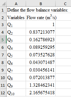
First define the variables that need to be found out: Flow rate
The variable definition is shown below:
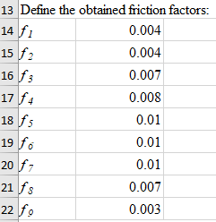
Next define the friction factors:
Step 2:
In each circular pipe length calculate the sectional pressure drop.
Consider the following formula for the pressure drop,
Here
Also,
And
With Q is the flow rate in
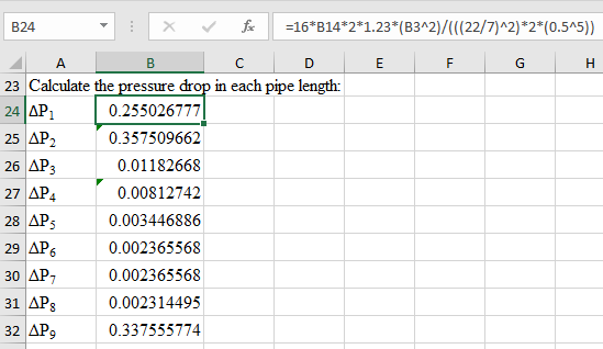
Note: The formula in the formula bar shows the Pressure calculation for
Now the pressure in other section of the pipes are calculated and shown in consequent cells with friction factor of
Step 3:
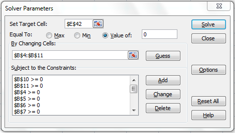
Constraint Setting:
Following are the required constraints or in other words the Equations to be solved:
And for pressure drops,
Also,
Since there is nothing to maximize or minimize, the pressure drop is the summation of three right hand loops, that is summation of cells: C28+C29+C30 is set to zero. In doing so, not only is the driving condition being set, but also no additional conditions are being added to alter the fate of the equations.
Once the arrangements are made, call Solver as shown below:
Continued after scroll down is shown below,
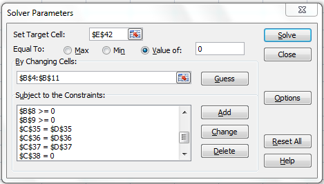
Next, click on Solve. The results are displayed below,
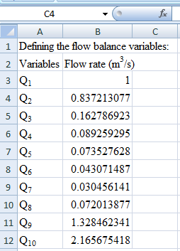
Therefore, the flows in each pipe length in
Want to see more full solutions like this?
Chapter 8 Solutions
EBK NUMERICAL METHODS FOR ENGINEERS
Additional Engineering Textbook Solutions
Fundamentals of Differential Equations (9th Edition)
Advanced Engineering Mathematics
Basic Technical Mathematics
Geometry, Student Edition
Linear Algebra and Its Applications (5th Edition)


- Fluid originally flows through a tube at a rate of 110 cm3 /s. To illustrate the sensitivity of flow rate to various factors, calculate the new flow rate for the following changes with all other factors remaining the same as in the original conditions.Randomized VariablesPx = 2.5ηx = 3.2rx = 0.14lx = 4.6Q = 110 cm3/s Part (a) Calculate the new flow rate in cm3/s if the pressure difference increases by a factor of 2.5 . Part (d) Calculate the new flow rate if another tube is used with a radius 0.14 times the original. Part (e) Calculate the new flow rate if yet another tube is substituted with a radius 0.14 times the original and half the length, and the pressure difference is increased by a factor of 2.5.arrow_forwardCalculations involving retention time involve the following formula, T =, where V is volume and Q is flow rate. Often times, you will be required to calculate the volume of more than one tank and determine a rate of flow, given a total retention time. Tank 1 Tank 2 Let's assume that the total retention time for the entire system is 55 minutes, and we want to know the inlet flow, given the dimensions of tank 1 are : 14m x 10m x 3 m, and tank 2 are: 5m x 10m x 3 m. Calculate the inlet flow.arrow_forwardThe pressure drop (Ap) test is carried out using a pipe configuration as illustrated below: Manometer 1 Manometer 2 straight pipe D= 2R R= radius in pipe The pipe data and the flowing fluid are as follows: Pipe: D = 1 cm; L= 100 cm. Fluid: Water, with density (A) = 1000 kg/m"; absolute viscosity (u) = 0.001 kg/im.s); Experimental data is shown as shown in the following table: Task: Ja. Plot the graph of the pressure as a function of the average velocity (V.v). b. Based on the equation for laminar flow in the pipe as follows: Ap = 32VuL, Vavg (m/s) Ap (Pa) 0,001 0,002 0,005 0,01 0,02 0,04 0,06 0,08 0,1 0,12 0,15 0,30 0,62 1,61 3,10 6,10 12,10 20,10 26,00 32,50 38,90 47,20 D Compare the experimental results in the table with the results of calculations using the above equation. Leave a comment. Note: Ap = p1-p2. c. The coefficient of friction (f) in the pipe is formulated as follows: f- 2DAD PL(V.) plot (plot) this distribution of fas a function of the Reynolds number (Re). Re is…arrow_forward
- Q.1 A simple and accurate viscometer can be made from a length of capillary tubing. If the flow rate and pressure drop are measured, and the tube geometry is known, the viscosity of Newtonian liquid can be computed. A test of a certain liquid in a capillary viscometer gave the following data: Flow rate: 880 mm /s, Tube length: 1 m, ,3, Tube diameter: 0.50 mm, Pressure drop: 1.0 MPа The viscosity of liquid will be (pig =999 kg/m:), assuming the flow to be laminar. A 0.37x10*Ns/m В 3.7x10* Ns/m 1.74x10* Ns/m C 1.74x10* Ns/marrow_forwardG1/ in the Pipe (A) is equal (PA= 25 Lit15), the diameter is equal ( DA - 75mm, Do = Fig.shown, the Flow rate in 6o mm, Dg = Dc%=30 mm), and the velocit Pipe (D) is equal (U0=5m/s), the relation between flow rate in Pipe (B) and pipe (c) %3D Find the Value af . 2- Un, UB, Uc. water Os = 30 mm input A QA - 25 Lit/sec = 75 mm fo mm %3D Inpud = A outPut = B,C,D accumule tion =o.arrow_forwardThree pipes A, B, and C are interconnected as shown in figure 1. The pipe dimensions are as follows: D (cm) 15 10 20 Pipeline A L (m) 300 240 600 0.01 0.01 0.005 A 15 m 25 m В C Figure 1 1.1 Find the rate at which water will flow in each pipe, ignoring the shock losses at P and entry to pipelines A and B. 1.2 Find the pressure at P.arrow_forward
- 7. An oil (sp.gr 0.9) is flowing through a 1.2m diameter pipe at a rate of 2.5 m³/s. The kinematic viscosity of oil is 3 X10⁶ m²/s. In order to model this flow, water is used to flow through a 120mm diameter pipe having kinematic viscosity of 0.012X10⁴ m²/s. Find the model discharge and velocity.arrow_forward7.58. A venturi meter is a device to measure fluid flow rates, which in its operation resembles the orifice meter (Section 3.2b). It consists of a tapered constriction in a line, with pressure taps leading to a differential manometer at points upstream of the constriction and at the point of maximum constriction (the throat). The manometer reading is directly related to the flow rate in the line. oment Encyclopedla tial pressure flowmeters/ venturi tube lley.com/college/felder * Adapted from a problem centributed by Justin Wood of North Carolina State University. Problems 399 Suppose the flow rate of an incompressible fluid is to be measured in a venturi meter in which the cross-sectional area at point 1 is four times that at point 2. (a) Derive the relationship between the velocities u¡ and u2 at points 1 and 2. (b) Write the Bernoulli equation for the system between points 1 and 2, and use it to prove that to the extenT friction is negligible 15 pv P - P2 = 247 where Pi and P2 are…arrow_forwardA well with 4 in. radius produces oil with a viscosity of0.3 cP, at a rate of 200 barrels/day, from a reservoir that is 15 ft.thick. The pressure in the wellbore as a function of time is: t (mins) 1 5 10 20 30 60 Pw(psi) 4740 4667 4633 4596 4573 4535 Use the "semi-log straight line" method to estimate the permeability, Karrow_forward
- The velocity distribution in a 0.02 m diameter horizontal pipe conveying carbon tetrachloride (specific gravity = 1.59, absolute viscosity = 9.6 x 10⁻⁶ Pa sec) is given by the parabolic equation: v(r)=0.01(0.12- r?), where v(r) is the velocity in (m/s) at a distance r in (m) from the pipe center. What is discharge? O a. 3.13 x-8 m3/s O b. None of the mentioned O c. 1.047 x 10⁸ m3/sec O d. 4.97 x 10⁹ m3/secarrow_forward7. a. If the blood viscosity is 2.7x10⁻³ Pa.s, length of the blood vessel is 0.35 m, tubular resistance of a blood vessel is 38.5 GPa-s/m3 , What is the radius of the blood vessel in mm?b. If the blood pressure at the outlet of the above vessel is 30 mm Hg and the flow rate through the vessel is 100 ml/min, find the inlet pressure in mm Hg. Density of mercury = 13,550 kg/m3, acceleration due to gravity = 9.61 m/s2arrow_forwardA storage tank contains a liquid at depth y where y= 0 when the tank is half full. Liquid is withdrawn at a constant flow rate Q to meet demands. The contents are resupplied at a sinusoidal rate 3Q sin'(t), The outflow is not constant but rather depends on the depth. For this case, the differential equation for depth is shown below. Some variable values are A = 1200 m?, Q = 500 m /d, and a (force function) = 300. Arrange the variables into the Mathematical Model format: stating which variable(s) is dependent, independent, etc. dy a(1+ y)15 dx A Figure P1.7arrow_forward
 Elements Of ElectromagneticsMechanical EngineeringISBN:9780190698614Author:Sadiku, Matthew N. O.Publisher:Oxford University Press
 Mechanics of Materials (10th Edition)Mechanical EngineeringISBN:9780134319650Author:Russell C. HibbelerPublisher:PEARSON
 Thermodynamics: An Engineering ApproachMechanical EngineeringISBN:9781259822674Author:Yunus A. Cengel Dr., Michael A. BolesPublisher:McGraw-Hill Education
 Control Systems EngineeringMechanical EngineeringISBN:9781118170519Author:Norman S. NisePublisher:WILEY
 Mechanics of Materials (MindTap Course List)Mechanical EngineeringISBN:9781337093347Author:Barry J. Goodno, James M. GerePublisher:Cengage Learning
 Engineering Mechanics: StaticsMechanical EngineeringISBN:9781118807330Author:James L. Meriam, L. G. Kraige, J. N. BoltonPublisher:WILEY