Control Systems Engineering
7th Edition
ISBN: 9781118170519
Author: Norman S. Nise
Publisher: WILEY
expand_more
expand_more
format_list_bulleted
Videos
Textbook Question
Chapter 7, Problem 43P
For each system shown in Figure P7.18, find the appropriate static error constant as well as the steady-state error, for unit step, ramp, and parabolic inputs. [Section: 7.6]
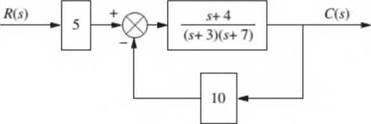
System 1
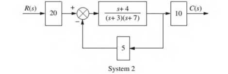
FIGURE P7.18
Expert Solution & Answer
Want to see the full answer?
Check out a sample textbook solution
Students have asked these similar questions
Q4) A particular control system yielded a steady state error of 0.20 for unit step input. A
unit integrator is cascaded to this system and unit ramp input is applied to this
modified system. What is the value of steady-state error for this modified system?
1 / 1
Problem No. 1
1A.
100% +
1B.
Consider the translational mechanical system shown
in Figure P4.17. A 1-pound force, f(t), is applied at
t = 0. If fy = 1, find K and M such that the response
is characterized by a 4-second settling time and a
1-second peak time. Also, what is the resulting
percent overshoot? [Section: 4.6]
70)
0000
31/1
10000
K
FIGURE P4.17
Given the translational mechanical system of
Figure P4.17, where K = 1 and f(1) is a unit step.
find the values of M and ƒ, to yield a response with
17% overshoot and a settling time of 10 seconds.
[Section: 4.6]
Feedback & Control Systems
State-Space Representation
Write the state-space representation of the system
below. Let the output of the mechanical system is
x3 (t).
1 N-s/m
x₁ (t) M3 = 1kg
1 N/m
М1
-0000 1kg
> X3 (t)
1 N-s/m
1 N/m
oooo
x₂ (t)
M₂
1kg
4
1 N-s/m²
-1 N-s/m
→f(t)
Chapter 7 Solutions
Control Systems Engineering
Ch. 7 - Prob. 1RQCh. 7 - A position control, tracking with a constant...Ch. 7 - Name the test inputs used to evaluate steady-state...Ch. 7 - Prob. 4RQCh. 7 - Increasing system gain has what effect upon the...Ch. 7 - Prob. 6RQCh. 7 - Prob. 7RQCh. 7 - Prob. 8RQCh. 7 - Prob. 9RQCh. 7 - The forward transfer function of a control system...
Ch. 7 - Prob. 11RQCh. 7 - Prob. 12RQCh. 7 - Is the forward-path actuating signal the system...Ch. 7 - Prob. 14RQCh. 7 - Prob. 15RQCh. 7 - Name two methods for calculating the steady-state...Ch. 7 - Prob. 1PCh. 7 - Figure P7.2 shows the ramp input r(t) and the...Ch. 7 - Prob. 3PCh. 7 - Prob. 4PCh. 7 - Prob. 5PCh. 7 - Prob. 6PCh. 7 - Prob. 7PCh. 7 - Prob. 8PCh. 7 - A system has Kp = 4. What steady-state error can...Ch. 7 - Prob. 10PCh. 7 - Prob. 11PCh. 7 - Prob. 12PCh. 7 - For the system shown in Figure P7.4. [Section:...Ch. 7 - Prob. 14PCh. 7 - 1515. Find the system type for the system of...Ch. 7 - Prob. 16PCh. 7 - Prob. 17PCh. 7 - Prob. 18PCh. 7 - Prob. 19PCh. 7 - Given the system of Figure P7.8, design the value...Ch. 7 - Prob. 21PCh. 7 - Prob. 22PCh. 7 - Prob. 23PCh. 7 - Prob. 24PCh. 7 - Prob. 25PCh. 7 - Prob. 26PCh. 7 - Prob. 27PCh. 7 - Prob. 28PCh. 7 - Prob. 29PCh. 7 - Prob. 30PCh. 7 - Prob. 31PCh. 7 - Prob. 32PCh. 7 - Given the system in Figure P7.9, find the...Ch. 7 - Repeat Problem 33 for the system shown in Figure...Ch. 7 - Prob. 36PCh. 7 - Prob. 37PCh. 7 - Prob. 38PCh. 7 - Design the values of K1and K2in the system of...Ch. 7 - Prob. 41PCh. 7 - For each system shown in Figure P7.17, find the...Ch. 7 - For each system shown in Figure P7.18, find the...Ch. 7 - Prob. 44PCh. 7 - 45. For the system shown in Figure P7.20,...Ch. 7 - Prob. 47PCh. 7 - Prob. 48PCh. 7 - Prob. 49PCh. 7 - Prob. 50PCh. 7 - Prob. 51PCh. 7 - Prob. 52PCh. 7 - Prob. 53PCh. 7 - Prob. 54PCh. 7 - Prob. 55PCh. 7 - Prob. 58PCh. 7 - Prob. 59PCh. 7 - Prob. 62PCh. 7 - Prob. 63PCh. 7 - Prob. 64PCh. 7 - Prob. 65PCh. 7 - Prob. 66PCh. 7 - Prob. 67PCh. 7 - Prob. 68P
Knowledge Booster


Learn more about
Need a deep-dive on the concept behind this application? Look no further. Learn more about this topic, mechanical-engineering and related others by exploring similar questions and additional content below.Similar questions
- The Routh-Hurwitz criterion to be used to determine the stability of a system with a characteristic equation given by 85 + 2s4 + 2s3 + 4s² + 11s + 10 Comment on the stability of the system. Neutral Stable Unstablearrow_forwardFor the system with open loop transfer function given by R(s) K s(s + 1) (s² + 4s +13) where K is the feedback gain. Sketch the root locus a) How many asymptotes are there for this system's root locus? what are asymptote angles? What is the center of asymptotes? C(s) b) Does the root locus cross the imaginary axis? where and what is the value of K at that point? c) Is there any break away, break in points? What is the approximate values of these points?arrow_forwardParameters of the following transfer function is given as: k=6, a=3.1, b=3.4, and c=2.8, determine the settling time Ts of the system response to a unit step input. (please keep four digits after decimal point) TF= k as²+bs+carrow_forward
- 11. Consider a system that can be modeled as shown. The input x in (t) is a prescribed motion at the right end of spring k 2. Find X(s) the system transfer function Xeq(s)* m k₂ ww Xin The values of the parameters are m= 30 kg, k ₁=700 N/m, k 2= 1300 N/m, and b=200 N- s/m. Write a MATLAB script file that: (a) calculates the natural frequency, damping ratio, and damped natural frequency for the system; and (b) uses the impulse command to find and plot the response of the system to a unit impulse input.arrow_forwardThe response to a unit step input (applied at time t = 0 s) of a system is shown in Figure Q2, determine the transfer function of this system from the step response graph. Amplitude 2.6 2.4 2.2 28 1.8 1.6 64 1.4 1.2 1 0.8 0.6 0.4 0.2 0 0 Step Response 0.1 0.2 0.3 0.4 0.5 0.6 0.7 0.8 0.9 1 1.1 Time (sec) Figure Q2 Step response 1.2arrow_forward(b) The response to a unit step input (applied at time t = 0 s) of a system is shown in Figure Q2, determine the transfer function of this system from the step response graph. Amplitude 2.6 2.4 2.2 2 1.8 1.6 1.4 1.2 1 0.8 0.6 0.4 0.2 0 0 Amplitude 5 Step input of 3 units was applied to a system and the response of this system is shown in Figure Q2.2. Determine the transfer function of this system. 4.5 4 3.5 3 2.5 2 1.5 1 0.5 0 o Step Response 0.1 0.2 0.3 0.4 0.5 0.6 0.7 0.8 0.9 1 1.1 1.2 Time (sec) Figure Q2 Step response Step Response 2 Time (seconds) 3arrow_forward
- Consider the following mechanical system: k m +f b d²y(t) +b- dy(t) + ky(t) = f (t) m %3D dt? dt Obtain the state space model of the system with input f (t) and output y(t). Calculate the system matrices for m = 1, k = 1 and b = 2. Check the stability by using the second method of Lyapunov. 3.arrow_forward6. Consider the mechanical system shown in Fig. 8. Let V(t) be the input and the acceleration of the mass be the output. Derive the state equations and the output equation using linear graphs and normal trees. B m V₁(t) Figure 8: A mechanical system with an across-variable sourcearrow_forwardP.4: R(s) + E(s) K(s+7) s(s+5)(5 + 8)(5 + 12) C(s) a. What value of K will yield a steady-state error in position of 0.01 for an input of (1/10)? b. What is the K, for the value of K found in (a)? c. What is the minimum possible steady-state position error for the input given in (a)? s(1/s²) e(00) = Cramp (00) = lim1+G(s) 1 05+sG(s) = lim 1 lim sG(s) 5-0arrow_forward
- 6. Given the system shown below, design a value of K so that for an input of 100tu(t), there will be a 0.01 steady-state error. R(s) K s(s + 1) 10s K C(s)arrow_forward2. Consider the state equation x1 1 20 x1 d x2 = 0 10 x2 dt x3 001 x3 where x1, x2 and 23 are state variables. Please answer the following questions. (a) The state matrix (4) 1 20 A = 0 1 0 (5) 0 0 1 has three-fold eigenvalues with \₁ = = A2 A3 1. Find all independent eigenvectors corresponding to this eigenvalue. (b) Find the modal matrix M associated with the state matrix A. Does M-1 AM lead to a Jordan form or not? Hint: The modal matrix M turns out to be a diagonal matrix. For a diagonal matrix, its inverse is given by a 00 0b0 -1 1/a 0 0 = 0 1/b 0 00 с 0 0 1/c 1 (6) (c) Find the state transition matrix (t). (d) Determine the stability of the system. Please justify your answer.arrow_forward1) a) Derive the mathematical model for the system shown below. b) Find a state variable model (matrix form) for the system. b) Determine state matrix, input matrix, and output matrix, when f (t) is defined as the input and X2 is defined as output for the system. (Here, both of the X1 and x2 , are time-dependent functions) » f(t) X1 X2 3,000 N 1,000 N 4,000 30 kg 20 kg 200 유 N.sarrow_forward
arrow_back_ios
SEE MORE QUESTIONS
arrow_forward_ios
Recommended textbooks for you
 Elements Of ElectromagneticsMechanical EngineeringISBN:9780190698614Author:Sadiku, Matthew N. O.Publisher:Oxford University Press
 Mechanics of Materials (10th Edition)Mechanical EngineeringISBN:9780134319650Author:Russell C. HibbelerPublisher:PEARSON
 Thermodynamics: An Engineering ApproachMechanical EngineeringISBN:9781259822674Author:Yunus A. Cengel Dr., Michael A. BolesPublisher:McGraw-Hill Education
 Control Systems EngineeringMechanical EngineeringISBN:9781118170519Author:Norman S. NisePublisher:WILEY
 Mechanics of Materials (MindTap Course List)Mechanical EngineeringISBN:9781337093347Author:Barry J. Goodno, James M. GerePublisher:Cengage Learning
 Engineering Mechanics: StaticsMechanical EngineeringISBN:9781118807330Author:James L. Meriam, L. G. Kraige, J. N. BoltonPublisher:WILEY
Elements Of Electromagnetics
Mechanical Engineering
ISBN:9780190698614
Author:Sadiku, Matthew N. O.
Publisher:Oxford University Press
Mechanics of Materials (10th Edition)
Mechanical Engineering
ISBN:9780134319650
Author:Russell C. Hibbeler
Publisher:PEARSON
Thermodynamics: An Engineering Approach
Mechanical Engineering
ISBN:9781259822674
Author:Yunus A. Cengel Dr., Michael A. Boles
Publisher:McGraw-Hill Education
Control Systems Engineering
Mechanical Engineering
ISBN:9781118170519
Author:Norman S. Nise
Publisher:WILEY
Mechanics of Materials (MindTap Course List)
Mechanical Engineering
ISBN:9781337093347
Author:Barry J. Goodno, James M. Gere
Publisher:Cengage Learning
Engineering Mechanics: Statics
Mechanical Engineering
ISBN:9781118807330
Author:James L. Meriam, L. G. Kraige, J. N. Bolton
Publisher:WILEY
Ficks First and Second Law for diffusion (mass transport); Author: Taylor Sparks;https://www.youtube.com/watch?v=c3KMpkmZWyo;License: Standard Youtube License