Control Systems Engineering
7th Edition
ISBN: 9781118170519
Author: Norman S. Nise
Publisher: WILEY
expand_more
expand_more
format_list_bulleted
Concept explainers
Videos
Textbook Question
Chapter 7, Problem 39P
Design the values of K1and K2in the system of Figure P7.15 to meet the following specifications: Steady-state error component due to a unit step disturbance is —0.00001; steady-state error component due to a unit ramp input is 0.002. [Section: 7.5J
D(s) 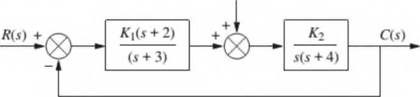
FIGURE P7.15
Expert Solution & Answer
Want to see the full answer?
Check out a sample textbook solution
Students have asked these similar questions
Feedback & Control Systems
State-Space Representation
Write the state-space representation of the system
below. Let the output of the mechanical system is
x3 (t).
1 N-s/m
x₁ (t) M3 = 1kg
1 N/m
М1
-0000 1kg
> X3 (t)
1 N-s/m
1 N/m
oooo
x₂ (t)
M₂
1kg
4
1 N-s/m²
-1 N-s/m
→f(t)
6. Given the system shown below, design a value of K so that for an input of 100tu(t), there will be a
0.01 steady-state error.
R(s)
K
s(s + 1)
10s
K
C(s)
The Routh-Hurwitz criterion to be used to determine the stability of a system with a characteristic equation given by
85 + 2s4 + 2s3 + 4s² + 11s + 10
Comment on the stability of the system.
Neutral
Stable
Unstable
Chapter 7 Solutions
Control Systems Engineering
Ch. 7 - Prob. 1RQCh. 7 - A position control, tracking with a constant...Ch. 7 - Name the test inputs used to evaluate steady-state...Ch. 7 - Prob. 4RQCh. 7 - Increasing system gain has what effect upon the...Ch. 7 - Prob. 6RQCh. 7 - Prob. 7RQCh. 7 - Prob. 8RQCh. 7 - Prob. 9RQCh. 7 - The forward transfer function of a control system...
Ch. 7 - Prob. 11RQCh. 7 - Prob. 12RQCh. 7 - Is the forward-path actuating signal the system...Ch. 7 - Prob. 14RQCh. 7 - Prob. 15RQCh. 7 - Name two methods for calculating the steady-state...Ch. 7 - Prob. 1PCh. 7 - Figure P7.2 shows the ramp input r(t) and the...Ch. 7 - Prob. 3PCh. 7 - Prob. 4PCh. 7 - Prob. 5PCh. 7 - Prob. 6PCh. 7 - Prob. 7PCh. 7 - Prob. 8PCh. 7 - A system has Kp = 4. What steady-state error can...Ch. 7 - Prob. 10PCh. 7 - Prob. 11PCh. 7 - Prob. 12PCh. 7 - For the system shown in Figure P7.4. [Section:...Ch. 7 - Prob. 14PCh. 7 - 1515. Find the system type for the system of...Ch. 7 - Prob. 16PCh. 7 - Prob. 17PCh. 7 - Prob. 18PCh. 7 - Prob. 19PCh. 7 - Given the system of Figure P7.8, design the value...Ch. 7 - Prob. 21PCh. 7 - Prob. 22PCh. 7 - Prob. 23PCh. 7 - Prob. 24PCh. 7 - Prob. 25PCh. 7 - Prob. 26PCh. 7 - Prob. 27PCh. 7 - Prob. 28PCh. 7 - Prob. 29PCh. 7 - Prob. 30PCh. 7 - Prob. 31PCh. 7 - Prob. 32PCh. 7 - Given the system in Figure P7.9, find the...Ch. 7 - Repeat Problem 33 for the system shown in Figure...Ch. 7 - Prob. 36PCh. 7 - Prob. 37PCh. 7 - Prob. 38PCh. 7 - Design the values of K1and K2in the system of...Ch. 7 - Prob. 41PCh. 7 - For each system shown in Figure P7.17, find the...Ch. 7 - For each system shown in Figure P7.18, find the...Ch. 7 - Prob. 44PCh. 7 - 45. For the system shown in Figure P7.20,...Ch. 7 - Prob. 47PCh. 7 - Prob. 48PCh. 7 - Prob. 49PCh. 7 - Prob. 50PCh. 7 - Prob. 51PCh. 7 - Prob. 52PCh. 7 - Prob. 53PCh. 7 - Prob. 54PCh. 7 - Prob. 55PCh. 7 - Prob. 58PCh. 7 - Prob. 59PCh. 7 - Prob. 62PCh. 7 - Prob. 63PCh. 7 - Prob. 64PCh. 7 - Prob. 65PCh. 7 - Prob. 66PCh. 7 - Prob. 67PCh. 7 - Prob. 68P
Knowledge Booster


Learn more about
Need a deep-dive on the concept behind this application? Look no further. Learn more about this topic, mechanical-engineering and related others by exploring similar questions and additional content below.Similar questions
- 11. Consider a system that can be modeled as shown. The input x in (t) is a prescribed motion at the right end of spring k 2. Find X(s) the system transfer function Xeq(s)* m k₂ ww Xin The values of the parameters are m= 30 kg, k ₁=700 N/m, k 2= 1300 N/m, and b=200 N- s/m. Write a MATLAB script file that: (a) calculates the natural frequency, damping ratio, and damped natural frequency for the system; and (b) uses the impulse command to find and plot the response of the system to a unit impulse input.arrow_forwardQ4) A particular control system yielded a steady state error of 0.20 for unit step input. A unit integrator is cascaded to this system and unit ramp input is applied to this modified system. What is the value of steady-state error for this modified system?arrow_forward4G I. 3:22 A moodle1.du.edu.om Consider the 3 degree of freedom robot manipulator as shown in the figure Link 3 Länk 2 Trint 1 The objective is to find the kinematics inverse of the robot Px=0.9 m, Py=0.6, L1=1.5m, L2=1.5m and qz= 2 rad The value of cos(q2) is equal to Choose... + The positive value of sin(q2) is equal to Choose... + The value of q2 in rad is Choose... + The value of qı in rad is Choose... + The value of q3 in rad is Choose... +arrow_forward
- My Solutions > Lower Colorado River (Problem 11.12 in Chapra) The Lower Colorado River consists of a series of four reservoirs as shown in Fig. P11.12 in the textbook. Mass balances can be written for each reservoir, and the following set of simultaneous linear algebraic equations results: [ 13.422 0 00; -13.422 12.252 0 0; 0 -12.252 12.377 0; 00-12.377 11.797] * [C_1, c_2, c_3, c_4]' = [750.5, 300, 102, 30] where the right-hand-side vector consists of the loadings of chloride to each of the four lakes. The variables c_1, c_2, c_3, and c_4 are the resulting chloride concentrations for Lakes Powell, Mead, Mohave, and Havasu, respectively. Given this information, complete the following tasks: (a) Use the matrix inverse to solve for the concentrations in each of the four lakes. (b) How much must the loading to Lake Powell be reduced for the chloride concentration of Lake Havasu to be 75? (c) Using the matrix 2-norm (spectral norm), compute the condition number and how many suspect digits…arrow_forwardP.4: R(s) + E(s) K(s+7) s(s+5)(5 + 8)(5 + 12) C(s) a. What value of K will yield a steady-state error in position of 0.01 for an input of (1/10)? b. What is the K, for the value of K found in (a)? c. What is the minimum possible steady-state position error for the input given in (a)? s(1/s²) e(00) = Cramp (00) = lim1+G(s) 1 05+sG(s) = lim 1 lim sG(s) 5-0arrow_forwardA velocity of a vehicle is required to be controlled and maintained constant even if there are disturbances because of wind, or road surface variations. The forces that are applied on the vehicle are the engine force (u), damping/resistive force (b*v) that opposing the motion, and inertial force (m*a). A simplified model is shown in the free body diagram below. From the free body diagram, the ordinary differential equation of the vehicle is: m * dv(t)/ dt + bv(t) = u (t) Where: v (m/s) is the velocity of the vehicle, b [Ns/m] is the damping coefficient, m [kg] is the vehicle mass, u [N] is the engine force. Question: Assume that the vehicle initially starts from zero velocity and zero acceleration. Then, (Note that the velocity (v) is the output and the force (w) is the input to the system): A. Use Laplace transform of the differential equation to determine the transfer function of the system.arrow_forward
- Parameters of the following transfer function is given as: k=6, a=3.1, b=3.4, and c=2.8, determine the settling time Ts of the system response to a unit step input. (please keep four digits after decimal point) TF= k as²+bs+carrow_forwardA velocity of a vehicle is required to be controlled and maintained constant even if there are disturbances because of wind, or road surface variations. The forces that are applied on the vehicle are the engine force (u), damping/resistive force (b*v) that opposing the motion, and inertial force (m*a). A simplified model is shown in the free body diagram below. From the free body diagram, the ordinary differential equation of the vehicle is: m * dv(t)/ dt + bv(t) = u (t) Where: v (m/s) is the velocity of the vehicle, b [Ns/m] is the damping coefficient, m [kg] is the vehicle mass, u [N] is the engine force. Question: Assume that the vehicle initially starts from zero velocity and zero acceleration. Then, (Note that the velocity (v) is the output and the force (w) is the input to the system): 1. What is the order of this system?arrow_forwardCharacteristic equation of a system is given by: C = s³ + 4s² + 25s + K = 0 %3D determine the range of values of K for which the system is stable. Use Roth Hurwitz stability criteria.arrow_forward
- O 1::09 O [Template] Ho... -> Homework For the system shown in figure below, Find the range of K for stable system. R K(s + 2) C s(s +5)(s² + 2s + 5) IIarrow_forwardR$ RL V (t) V(t) L Figure 7: A tuning circuit for radio 5. Figure 7 shows a tuning circuit used in radio. Derive the state equation using the linear graph approach. Also let the output variable be the voltage vo(t). Derive the output equation.arrow_forwardConsider the following Initial Value Problem (IVP) dy /at = -t * sin (y); y(t = 0) =1 Solve for y(t=0.5) using a) Forward Euler method with At = 0.25. (Solve by hand) Develop a Matlab script that solves for y (t = 5) using Forward Euler method. Use the time step levels given below and plot t vs y in the same plot. Include the plot with the right format (axis labels, legends, ...) in your solution sheet and include your Matlab script in the solution as well. i) At = 0.25 ii) At = 0.125 b) Backward Euler method with At = 0.25 (Solve by hand)arrow_forward
arrow_back_ios
SEE MORE QUESTIONS
arrow_forward_ios
Recommended textbooks for you
 Elements Of ElectromagneticsMechanical EngineeringISBN:9780190698614Author:Sadiku, Matthew N. O.Publisher:Oxford University Press
 Mechanics of Materials (10th Edition)Mechanical EngineeringISBN:9780134319650Author:Russell C. HibbelerPublisher:PEARSON
 Thermodynamics: An Engineering ApproachMechanical EngineeringISBN:9781259822674Author:Yunus A. Cengel Dr., Michael A. BolesPublisher:McGraw-Hill Education
 Control Systems EngineeringMechanical EngineeringISBN:9781118170519Author:Norman S. NisePublisher:WILEY
 Mechanics of Materials (MindTap Course List)Mechanical EngineeringISBN:9781337093347Author:Barry J. Goodno, James M. GerePublisher:Cengage Learning
 Engineering Mechanics: StaticsMechanical EngineeringISBN:9781118807330Author:James L. Meriam, L. G. Kraige, J. N. BoltonPublisher:WILEY
Elements Of Electromagnetics
Mechanical Engineering
ISBN:9780190698614
Author:Sadiku, Matthew N. O.
Publisher:Oxford University Press
Mechanics of Materials (10th Edition)
Mechanical Engineering
ISBN:9780134319650
Author:Russell C. Hibbeler
Publisher:PEARSON
Thermodynamics: An Engineering Approach
Mechanical Engineering
ISBN:9781259822674
Author:Yunus A. Cengel Dr., Michael A. Boles
Publisher:McGraw-Hill Education
Control Systems Engineering
Mechanical Engineering
ISBN:9781118170519
Author:Norman S. Nise
Publisher:WILEY
Mechanics of Materials (MindTap Course List)
Mechanical Engineering
ISBN:9781337093347
Author:Barry J. Goodno, James M. Gere
Publisher:Cengage Learning
Engineering Mechanics: Statics
Mechanical Engineering
ISBN:9781118807330
Author:James L. Meriam, L. G. Kraige, J. N. Bolton
Publisher:WILEY
What is Metrology in Mechanical Engineering? | Terminologies & Measurement; Author: GaugeHow;https://www.youtube.com/watch?v=_KhMhFRehy8;License: Standard YouTube License, CC-BY