Nonlinear Dynamics and Chaos
2nd Edition
ISBN: 9780813349107
Author: Steven H. Strogatz
Publisher: PERSEUS D
bartleby

Videos

Question
Book Icon
Chapter 6.6, Problem 6E
Interpretation Introduction

Interpretation:

To plot the nullclines x˙ = 0 and y˙ = 0 for the system x˙ = y - y3, y˙ = - x - y2. To find the sign of x˙y˙ in different regions of the plane. To find the Eigenvalues and Eigenvectors of the saddle points at (-1, ±1). To prove that the unstable manifold (-1, -1) intersects the negative x- axis. To use reversibility to prove the existence of a heteroclinic trajectory connecting (-1, -1) to (-1, 1). To prove that another heteroclinic trajectory exists and to sketch several other trajectories to fill in the phase portrait.

Concept Introduction:

Nullclines are the curves in the phase portrait where either x˙ = 0 or y˙ = 0.

Fixed points occur where x˙ = 0 and y˙ = 0.

The Jacobian matrix at a general point (x, y) is given by

J = (x˙xx˙yy˙xy˙y)

The Eigenvalue λ can be calculated using the characteristic equation

|(A - λI)| = 0

The solution of the quadratic equation is λ = -b ± b2- 4ac2a

The unstable manifold for a fixed point is the set of all points in the plane which tend to the fixed point as time goes to negative infinity.

Expert Solution & Answer
Check Mark

Answer to Problem 6E

Solution:

a) The nullclines x˙ = 0 and y˙ = 0 for the given system are plotted.

b) The sign of x˙ and y˙ in different regions of the plane is shown in the nullcline plot.

c) The Eigenvalues and Eigenvectors of the saddle points at (-1, ±1) are calculated.

d) It is proved that the unstable manifold (-1, -1) intersects the negative x- axis. It is proved that the heteroclinic trajectory exists, connecting (-1, -1) to (-1, 1).

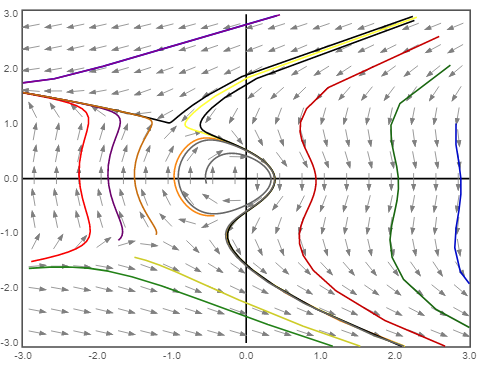
e) The phase portrait for the given system is plotted.

Explanation of Solution

a) The system is given as

x˙ = y - y3, y˙ = - x - y2

Nullclines are the curves in the phase portrait where either x˙ = 0 or y˙ = 0.

Substituting x˙ = 0 in the above system,

y - y3 = 0

y(1 - y2) = 0

y = 0 and (1 - y2) = 0  y = ±1

Thus,

y = 0, 1, -1.

Substituting y˙ = 0 in the above system,

- x - y2 = 0y = ±-x

Therefore, the nullclines of the given system are

y = 0, 1, -1y = ±-x

The nullclines plot for the given system equation is shown below:

Nonlinear Dynamics and Chaos, Chapter 6.6, Problem 6E , additional homework tip  1

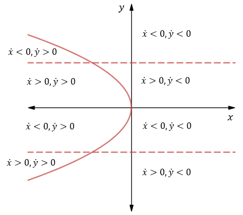
b) The value of the system at x˙ and y˙ lie in all the four quadrants, and it depends on the value of the initial conditions of the system.

The sign of x˙ and y˙ in different regions of the plane is shown in the above nullcline plot.

c) The fixed points of the system would be where x˙ = 0 and y˙ = 0.

The fixed points can be obtained by substituting x˙ = 0 and y˙ = 0 in the given system.

Therefore, the fixed points are (0, 0) (-1, 1) and (-1, -1).

The Jacobian matrix at a general point (x, y) is given by

J = (x˙xx˙yy˙xy˙y)

Substituting the given system in the Jacobian matrix,

J = ((y - y3)x(y - y3)y(- x - y2)x(- x - y2)y)

J = (01 - 3y2-1- 2y)

The value of the Jacobian matrix at the fixed point (0, 0) is

J(0, 0) = (01-10)

Therefore, from the Jacobian matrix, it is clear that the fixed point (0, 0) is a clockwise center.

The value of the Jacobian matrix at the fixed point (-1, 1) is

J(-1, 1) = (0-2-1-2)

The value of the Jacobian matrix at the fixed point (-1, -1) is

J(-1, 1) = (0-2-12)

The Eigenvalue λ can be calculated using the characteristic equation

|(A - λI)| = 0

To find the Eigenvalues and the Eigenvectors of the Jacobian matrix J(-1,1), substitute J = (0-2-1-2) and I = (1001),

(0-2-1-2) - λ(1001) = 0

(-2-1-2 - λ) = 0

The determinant of the above matrix is

Δ(-1,1) = -λ(-2 - λ) - 2

From the above matrix,

λ2 + 2λ - 2 = 0

The above quadratic equation can be solved by using λ = -b ± b2- 4ac2a

λ = -2 ± 22-(4)(-2)2

λ = -1 ± 3

Therefore, the Eigenvalue of the Jacobian matrix J(-1, 1) is λ = -1 ± 3

The corresponding Eigenvectors for the above Jacobian matrix J(-1, 1) are

v1 = (11 - 32)v2 = (11 + 32)

Similarly, to find the Eigenvalues and the Eigenvectors of the Jacobian matrix J(-1, -1), substitute J = (0-2-12) and I = (1001),

(0-2-12) - λ(1001) = 0

(-2-12 - λ) = 0

The determinant of the above matrix is

Δ(-1, -1) = -λ(2 - λ) - 2

From the above matrix,

λ2 - 2λ - 2 = 0

The above quadratic equation can be solved by using λ = -b ± b2- 4ac2a

λ = - (-2) ± (-2)2-(4)(-2)2

λ = 1 ± 3

Therefore, the Eigenvalue of the Jacobian matrix J(-1, -1) is λ = 1 ± 3

The corresponding Eigenvectors for the above Jacobian matrix J(-1, -1) are

v1 = (11 - 3-2)v2 = (11 + 3-2)

d) The unstable manifold for a fixed point is the set of all points in the plane which tend to the fixed point as time goes to negative infinity.

Consider the unstable manifold of the saddle point (-1, -1). The part of the unstable manifold lies in the region where x˙ < 0, y˙ > 0. A phase point along the manifold will move up and to the left and eventually will cut the negative x- axis.

Since the system is reversible under the transformation t -t, y -y. By reversibility, there must be a twin trajectory with the same endpoint on the negative x- axis from (1, 1) but with arrow reversed. Together the two trajectories form a heteroclinic orbit.

e) Consider the unstable manifold of the saddle point (-1, 1). The part of the unstable manifold lies in the region where x˙ > 0, y˙ < 0. A phase point along the manifold will move down and to the right and eventually will cut the positive x- axis.

Since the system is reversible under the transformation t -t, y -y. By reversibility, there must be a twin trajectory with the same endpoint on the positive x- axis from (1, -1) but with arrow reversed. Together the two trajectories form another heteroclinic orbit.

The phase portrait of the given system is shown below:

Nonlinear Dynamics and Chaos, Chapter 6.6, Problem 6E , additional homework tip  2

Want to see more full solutions like this?

Subscribe now to access step-by-step solutions to millions of textbook problems written by subject matter experts!

Chapter 6 Solutions

Nonlinear Dynamics and Chaos

Ch. 6.1 - Prob. 11ECh. 6.1 - Prob. 12ECh. 6.1 - Prob. 13ECh. 6.1 - Prob. 14ECh. 6.2 - Prob. 1ECh. 6.2 - Prob. 2ECh. 6.3 - Prob. 1ECh. 6.3 - Prob. 2ECh. 6.3 - Prob. 3ECh. 6.3 - Prob. 4ECh. 6.3 - Prob. 5ECh. 6.3 - Prob. 6ECh. 6.3 - Prob. 7ECh. 6.3 - Prob. 8ECh. 6.3 - Prob. 9ECh. 6.3 - Prob. 10ECh. 6.3 - Prob. 11ECh. 6.3 - Prob. 12ECh. 6.3 - Prob. 13ECh. 6.3 - Prob. 14ECh. 6.3 - Prob. 15ECh. 6.3 - Prob. 16ECh. 6.3 - Prob. 17ECh. 6.4 - Prob. 1ECh. 6.4 - Prob. 2ECh. 6.4 - Prob. 3ECh. 6.4 - Prob. 4ECh. 6.4 - Prob. 5ECh. 6.4 - Prob. 6ECh. 6.4 - Prob. 7ECh. 6.4 - Prob. 8ECh. 6.4 - Prob. 9ECh. 6.4 - Prob. 10ECh. 6.4 - Prob. 11ECh. 6.5 - Prob. 1ECh. 6.5 - Prob. 2ECh. 6.5 - Prob. 3ECh. 6.5 - Prob. 4ECh. 6.5 - Prob. 5ECh. 6.5 - Prob. 6ECh. 6.5 - Prob. 7ECh. 6.5 - Prob. 8ECh. 6.5 - Prob. 9ECh. 6.5 - Prob. 10ECh. 6.5 - Prob. 11ECh. 6.5 - Prob. 12ECh. 6.5 - Prob. 13ECh. 6.5 - Prob. 14ECh. 6.5 - Prob. 15ECh. 6.5 - Prob. 16ECh. 6.5 - Prob. 17ECh. 6.5 - Prob. 18ECh. 6.5 - Prob. 19ECh. 6.5 - Prob. 20ECh. 6.6 - Prob. 1ECh. 6.6 - Prob. 2ECh. 6.6 - Prob. 3ECh. 6.6 - Prob. 4ECh. 6.6 - Prob. 5ECh. 6.6 - Prob. 6ECh. 6.6 - Prob. 7ECh. 6.6 - Prob. 8ECh. 6.6 - Prob. 9ECh. 6.6 - Prob. 10ECh. 6.6 - Prob. 11ECh. 6.7 - Prob. 1ECh. 6.7 - Prob. 2ECh. 6.7 - Prob. 3ECh. 6.7 - Prob. 4ECh. 6.7 - Prob. 5ECh. 6.8 - Prob. 1ECh. 6.8 - Prob. 2ECh. 6.8 - Prob. 3ECh. 6.8 - Prob. 4ECh. 6.8 - Prob. 5ECh. 6.8 - Prob. 6ECh. 6.8 - Prob. 7ECh. 6.8 - Prob. 8ECh. 6.8 - Prob. 9ECh. 6.8 - Prob. 10ECh. 6.8 - Prob. 11ECh. 6.8 - Prob. 12ECh. 6.8 - Prob. 13ECh. 6.8 - Prob. 14E
Knowledge Booster
Background pattern image
Advanced Math
Learn more about
Need a deep-dive on the concept behind this application? Look no further. Learn more about this topic, advanced-math and related others by exploring similar questions and additional content below.
Recommended textbooks for you
Text book image
Linear Algebra: A Modern Introduction
Algebra
ISBN:9781285463247
Author:David Poole
Publisher:Cengage Learning
Lecture 46: Eigenvalues & Eigenvectors; Author: IIT Kharagpur July 2018;https://www.youtube.com/watch?v=h5urBuE4Xhg;License: Standard YouTube License, CC-BY
What is an Eigenvector?; Author: LeiosOS;https://www.youtube.com/watch?v=ue3yoeZvt8E;License: Standard YouTube License, CC-BY