Concept explainers
a.
To calculate: The dollar sales of ice cream in two years, based on the regression equation treating ice cream sales as the dependent variable and time as the independent variable
Introduction: Regression analysis is a statistical method for estimating the interactions between variables. In data
a.
Answer to Problem 54AP
The dollar sales of ice cream in two years:
Explanation of Solution
| Month | Park Attendies | Ice cream sales | ||
| 1 | 880 | 325 | 286,000 | 77,440 |
| 2 | 976 | 335 | 326,926 | 95,576 |
| 3 | 440 | 172 | 75,680 | 193,600 |
| 4 | 1,823 | 645 | 1,175,835 | 3,323,329 |
| 5 | 1,885 | 770 | 1,451,450 | 3,553,225 |
| 6 | 2,436 | 950 | 2,314,200 | 5,934,096 |
| Total = 21 | 8440 | 3197 | 5,630,125 | 13,177,266 |
Substituting the values in equation (1)
Calculating general regression using the following equations:
Now,
Calculating the regression equation below:
The forecast predicted does not seem confident enough to assume as the trend observed over the first six months might be unlikely for the next six months of the year.
b.
To calculate: A regression equation treating ice cream sales as the dependent variable and part attendees as the independent variable
Introduction: Regression analysis is a statistical method for estimating the interactions between variables. In data forecasting, companies can learn trends using regression analysis. It enables data based predictions to be made.
b.
Answer to Problem 54AP
Explanation of Solution
| Month | Park Attendies | Ice cream sales | ||
| 1 | 880 | 325 | 286,000 | 77,440 |
| 2 | 976 | 335 | 326,926 | 95,576 |
| 3 | 440 | 172 | 75,680 | 193,600 |
| 4 | 1,823 | 645 | 1,175,835 | 3,323,329 |
| 5 | 1,885 | 770 | 1,451,450 | 3,553,225 |
| 6 | 2,436 | 950 | 2,314,200 | 5,934,096 |
| Total = 21 | 8440 | 3197 | 5,630,125 | 13,177,266 |
Substituting the values in equation (3)
Calculating general regression using the following equations:
Now,
c.
To calculate: Ice cream sales for months 12 through 18, based on the curve and the regression equation determined in part (b)
Introduction: Regression analysis is a statistical method for estimating the interactions between variables. In data forecasting, companies can learn trends using regression analysis. It enables data based predictions to be made.
c.
Answer to Problem 54AP
Explanation of Solution
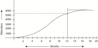
The following logistic curve can be considered for obtaining values:

The number of attendies observed from the logistic curve from months 12 to 18 until peak 3000 is shown below:
| MONTH | ATTENDIES | PREDICTED ICE CREAM SALES |
| 12 | 5100 | 1995.39 |
| 13 | 5350 | 2094.39 |
| 14 | 5600 | 2193.39 |
| 15 | 5800 | 2272.59 |
| 16 | 5900 | 2312.19 |
| 17 | 5950 | 2331.99 |
| 18 | 5980 | 2343.87 |
Using the regression equation
Want to see more full solutions like this?
Chapter 2 Solutions
Production and Operations Analysis, Seventh Edition
- provide schoarly research and references as to how internal and exteral audit is a risk management strategy to mitigate risk in a financial institutionarrow_forwardLearning Activity 4: Strategic Sales Management How has the advent and rapid evolution of digital technology transformed traditional sales management strategies, and what do you think are the most significant challenges and opportunities this transformation brings? In addition, please select and describe an example of company that has embraced change and implemented a unique and effective sales strategy.arrow_forward1) View the two video excerpts (Ctrl+Click on the two links), Preview 1 to the Goal Movie (Goldratt) (11.17 minutes), https://www.youtube.com/watch?v=2RVMgV37O_k and Preview 2 to the Goal Movie – How to Version (Goldratt) (9.40 minutes) https://www.youtube.com/watch?v=t_oM9LvK0rU and answer the following questions: a) What problems is UniCo facing and how are they tackling these problems currently? b) What advice did Jonah give to Rogo, and what lessons did Rogo learn from “Herbie’s Hike”? c) How do you think Rogo can leverage Jonah’s advice (as well as the lessons learnt from “Herbie’s Hike”) to solve UniCo’s problems? 2) A business program has the facilities and faculty to handle an enrollment of 2,000 new students per semester. However, in an effort to limit class sizes to a “reasonable” level the business dean, placed a ceiling on enrollment of 1,500 new students. Although there was ample demand for business courses last semester, conflicting schedules allowed only 1,450 new…arrow_forward
- The global marketplace has undergone a dramatic transformation, demanding that businesses adapt their supply chain management and implement new strategies to ensure the reliable sourcing of materials and goods. Please choose an organisation that you are currently working for or you are familiar with where its procurement operations has been greatly affected. You may pick a commercial or public institution as a choice for your study. You will need to briefly describe the institution and explain its category management structure which support the strategic procurement. You are required to provide an overview and discuss how spend are identified along with the types of categories purchased Briefly describe the organisation that you have chosen. Analyse the criticality of both the category management and strategic sourcing that will impact the business needs of the institution that you have chosen. Laing oxemples from the institution you have selected appraise and recommend COarrow_forwardThe Ideal Spot in the Segment Circles So, where should you try to position your product in the segment circles? As a basic rule, the 'Ideal Spot' will help guide you. The ideal spot represents the position with the highest point of demand for each consumer base – or segment. The ideal spot is made up by the product’s performance (speed) and size. As the perceptual map drifts down and to the right each year, the ideal spot will change as customers demand sensors with decreased size (smaller) and increased performance (faster). Although it would seem that the Ideal Spot would be in the center of the segment circle, the positioning actually varies due to the customer focus of each segment. For example, in the High End segment, the Ideal Spot is at the leading edge of the segment because those customers want the best possible product. Each segment’s ideal spot is represented by the pink dots on the Perceptual Map. Ideal Spots offset from segment center Calculating the Ideal Spot To…arrow_forwardIn Ecuador, cut roses are one of the country’s leading exports. Prior to advancements in the air transportation industry, this would have been impossible as roses must be sold within three to five days once cut. Today Ecuador is one of the world’s top producers of roses.arrow_forward
- The World Trade Organization is the only global trade organization and has 164 member nations representing 98 percent of world trade. How does the WTO help nations improve trade relations? What are some of the major challenges facing the WTO today?arrow_forwardWhat is a good example of a letter of recommendation for a 5th grade Language Arts Teaching Position at an elementary school from a school principal?arrow_forwardProblem 1 (10 Points) Davison Electronics manufactures three LED television monitors, identified as Model A, Model B, and Model C. Davison Electronics four manufacturing plants. Each model has its lowest possible production cost when produced at Plant 1. However, Plant 1 does not have the capacity to handle the total production of all three models. As a result, at least some of the production must be routed to the other manufacturing plants. The following table shows the minimum production requirements for next month, the plant capacities in units per month, and the production cost per unit at each plant: Model Production Cost per Unit Minimum Production Requirements Plant 1 Plant 2 Plant 3 Plant 4 A $25 $28 $37 $34 48,000 B $26 $35 $36 $41 75,000 C $20 $31 $26 $23 60,000 Production Capacity 65,000 50,000 32,000 43,000 Davison’s objective is to determine the cost-minimizing production plan. We have…arrow_forward
- Lead Story: Identify the key story or insight based on your visualizations. Shaffer’s 4C Framework: Describe how you applied Shaffer’s 4C principles in the design of your charts. Gestalt Principles or Preattentive Attributes: Explain how you applied at least one Gestalt principle or preattentive attribute in your chartarrow_forwardFor the purpose of process analysis, which of the following measures would be considered an appropriate flow unit for analyzing the main operation of a local accounting firm? Instructions: You may select more than one answer. a. Number of accountants working each week b. Number of tax returns completed each week c. Number of customers with past-due invoices d. Number of reams of paper received from suppliersarrow_forward4. Based on the data provided in Table 2.5, what is the flow rate of callers from 8:00 a.m. to 8:20 a.m.? TABLE 2.5 Time Stamps of the Eight Callers Who Called from 8:00 a.m. to 8:20 a.m. to the Reservation Desk of a Ferry Service Caller Time In Time Out 1 8:01 8:05 2 3 4 5 6 8:02 8:07 8:06 8:08 8:09 8:12 8:10 8:15 8:12 8:20 7 8:16 8:19 8 8:17 8:19 5. Based on the data provided in Table 2.5, what is the flow time of callers from 8:00 a.m. to 8:20 a.m.? 6. Based on the data provided in Table 2.6, what is the flow rate of customers from 9:00 a.m. to 10:00 a.m.? TABLE 2.6 Time Stamps of 10 Customers Who Visited a Local Bank Branch from 9:00 a.m. to 10:00 a.m. Customer 1 2 3 4 5 6 7 8 9 10 Time In Time Out 9:01 9:07 9:06 9:21 9:08 9:20 9:14 9:19 9:20 9:28 9:26 9:33 9:31 9:39 9:40 9:46 9:44 9:59 9:53 9:57 7. Based on the data provided in Table 2.6, what is the flow time of customers from 9:00 a.m. to 10:00 a.m.?arrow_forward
 Practical Management ScienceOperations ManagementISBN:9781337406659Author:WINSTON, Wayne L.Publisher:Cengage,
 Contemporary MarketingMarketingISBN:9780357033777Author:Louis E. Boone, David L. KurtzPublisher:Cengage LearningMarketingMarketingISBN:9780357033791Author:Pride, William MPublisher:South Western Educational Publishing


