Chapter 18, Problem 8E

(a)

To determine

To explain why it is appropriate to use a normal model to describe the distribution of the proportion of green M&M’s they might expect.

Explanation of Solution

In the question, the candy company claims that $10\%$ of the M&M’s it produces are green. Suppose that the candies are packed at random in small bags. Then, the class of elementary school opens the bags and count the proportion that are green candies. Now, the class buys bigger bags of candies with each $200$ M&Ms. Thus, in the randomization condition: The $200$ M&Ms are considered representative and are thoroughly mixed. And for the $10\%$ condition: $200$ is less than $10\%$ of the population. And also,

  $\begin{array}{l}np=200(0.1)\\ =20\\ n(1-p)=200(0.9)\\ =180\end{array}$

Thus, these are both greater than ten and thus success/failure condition is also satisfied. So, all the conditions of normal model are met. Thus, it is appropriate to use a normal model to describe the distribution of the proportion of green M&M’s they might expect.

(b)

To determine

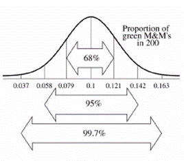
To use the rule $68-95-99.7$ to describe how this proportion might vary from bag to bag.

Explanation of Solution

In the question, the candy company claims that $10\%$ of the M&M’s it produces are green. Suppose that the candies are packed at random in small bags. Then, the class of elementary school opens the bags and count the proportion that are green candies. Now, the class buys bigger bags of candies with each $200$ M&Ms. Thus, using the rule $68-95-99.7$ , we get,

  $\begin{array}{l}\mu =p=0.1\\ \sigma =\sqrt{\frac{pq}{n}}\\ =\sqrt{\frac{0.1(0.9)}{200}}\\ =0.021\end{array}$

Thus, about $68\%$ of the sample proportions are expected to be between $\text{0}\text{.079 and 0}\text{.121}$ and about $95\%$ are expected to be between $\text{0}\text{.058 and 0}\text{.142}$ and about $99.7\%$ are expected to be between $\text{0}\text{.037 and 0}\text{.163}$ , by using the rule $68-95-99.7$ to describe the sampling distribution model. Thus, the diagram for this model is as:

  

(c)

To determine

To explain how this model change if the bags contained even more candies.

Answer to Problem 8E

The sampling distribution would also be less spread out.

Explanation of Solution

In the question, the candy company claims that $10\%$ of the M&M’s it produces are green. Suppose that the candies are packed at random in small bags. Then, the class of elementary school opens the bags and count the proportion that are green candies. Now, the class buys bigger bags of candies with each $200$ M&Ms. As we know that sample proportion is always equal to population proportion. But sine sample size increases, variability decreases, also decreasing standard deviation and spread. Thus, if the bags contained more candies, the sampling distribution would still be normal and centered at $0.1$ , but the standard deviation would decrease. The sampling distribution would also be less spread out.