Chapter 18, Problem 7E

(a)

To determine

To use the rule $68-95-99.7$ to describe the sampling distribution model.

Explanation of Solution

It is given in the question, the professor in the class has each person toss a coin $25$ times and calculate the proportion of his or her tosses that were heads. And the results of the students are plotted by a histogram by the professor of these several proportions. Since we know that the probabilities of the toss to be head and to be tail is equal in proportions as half. Now, as we know that,

  $\begin{array}{l}\mu =p=0.5\\ \sigma =\sqrt{\frac{pq}{n}}\\ =\sqrt{\frac{0.5(0.5)}{25}}\\ =0.1\end{array}$

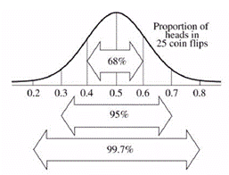
Thus, about $68\%$ of the sample proportions are expected to be between $0.4\text{ and 0}\text{.6}$ and about $95\%$ are expected to be between $0.3\text{ and 0}\text{.7}$ and about $99.7\%$ are expected to be between $0.2\text{ and 0}\text{.8}$ , by using the rule $68-95-99.7$ to describe the sampling distribution model. Thus, the diagram for this model is as:

  

(b)

To determine

To confirm that you can use normal model here.

Answer to Problem 7E

Yes, the normal model can be used here.

Explanation of Solution

It is given in the question, the professor in the class has each person toss a coin $25$ times and calculate the proportion of his or her tosses that were heads. And the results of the students are plotted by a histogram by the professor of these several proportions. Since we know that the probabilities of the toss to be head and to be tail is equal in proportions as half. Now, you can use the normal model here because all coin flips are independent, so there is no need to check the $10\%$ condition. Additionally the success/failure condition is met. Which can be verified by calculating:

  $\begin{array}{l}np=n(1-p)\\ =25(0.5)\\ =12.5>10\end{array}$

(c)

To determine

To check the appropriate condition to justify your model.

Explanation of Solution

It is given in the question, the professor in the class has each person toss a coin $25$ times and calculate the proportion of his or her tosses that were heads. And the results of the students are plotted by a histogram by the professor of these several proportions. Since we know that the probabilities of the toss to be head and to be tail is equal in proportions as half. Now, if they increase the number of tosses to $64$ each then,

  $\begin{array}{l}\mu =p=0.5\\ \sigma =\sqrt{\frac{pq}{n}}\\ =\sqrt{\frac{0.5(0.5)}{64}}\\ =0.0625\end{array}$

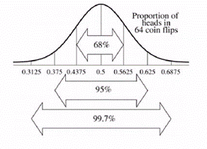
Thus, now we know that about $68\%$ of the sample proportions are expected to be between $\text{0}\text{.4375 and 0}\text{.5626}$ and about $95\%$ are expected to be between $\text{0}\text{.375 and 0}\text{.625}$ and about $99.7\%$ are expected to be between $\text{0}\text{.3125 and 0}\text{.6875}$ , by using the rule $68-95-99.7$ to describe the sampling distribution model. Thus, the diagram for this model is as:

  

(d)

To determine

To explain how the sampling distribution model changes as the number of tosses increases.

Answer to Problem 7E

As the number of tosses increases, sampling distribution will be less spread out.

Explanation of Solution

It is given in the question, the professor in the class has each person toss a coin $25$ times and calculate the proportion of his or her tosses that were heads. And the results of the students are plotted by a histogram by the professor of these several proportions. Since we know that the probabilities of the toss to be head and to be tail is equal in proportions as half. As we know that sample proportion is always equal to the population proportion. And as the sample size increases, variability decreases, resulting in the smaller standard deviation and spread. So, as the number of tosses increases, the sampling distribution will still be normal and centered at $0.5$ , but the standard deviation will decrease. The sampling distribution will be less spread out.